2021 paper

Yoonwoo Jeong
Seokjun Ahn Christopher Choy

---

• Abstract
• 1.Introduction
• 2. Related Work
• 3.Preliminary
• 4. Differentiable Self-Calibration Cameras
• 4.1 Differentiable Pinhole Camera Rays
• 4.1 Generic Non-Linear Ray Distortion
• 5. Geometric and Photometric Consistency
• Geom. Consistency: Projected Ray Distance
• 5.2 Chirality Check
• Photometric Consistency
• 6. Optimizing Geometry and Camera
• 6.1 Curriculum learning
• 6.2. Joint OPtimization
• 7. Experiment
• 7.1 Dataset
• 7.2 Self-Calibration

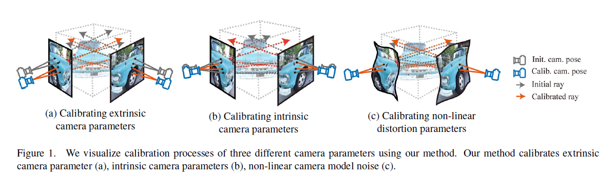
Figure1 : 우리는 우리의 방법을 이용하여 3개의 서로다른 camera parameters의 calibration 과정을 시각화하였다. 우리의 method는 extrinsic camera parameter (a)아 intrinsic camera parameters (b) 그리고 non-linear camera model noise (c)를 calibrates한다.

Abstract

arbitrary non-linear distortions을 갖는 일반적인 cameras에 대한 camera self-calibration algorithm을 제안한다. 우리는 어떠한 calibration objects 없이 scene의 geometry와 정확한 camera parameters를 jointly하게 학습한다. 우리의 camera model은 pinhole model, a fourth order radial distorthion 그리고 arbitrary non-linear camera distortions를 학습할 수 있는 generic noise model로 구성되어 있다. traditional self-calibration algorithms은 거의 대부분 geometric constraints에 의존하는 반면, 우리는 추가적으로 photometric consistency를 추가하였다. 그것은 scene의 geometry를 학습하는것을 요구하고 우리는 Neural Radiance Fields (NeRF)를 사용한다.

우리는 또한 complex non-linear camera models에 대해 geometric consistency를 통합하기 위해서 projected ray distance loss라는 새로운 geometric loss function을 제안한다.
우리는 standard real image datasets에 대해 우리의 approach를 calidate하고 우리의 model이 COLMAP initialization 없이 밑바닥부터 camera intrinsics와 extrinsics (pose)를 학습할 수 있음을 시연한다. 또한 우리는 미분가능한 방식으로 accurate camera models를 학습하는것이 baseline보다 PSNR을 향상시킬수 있게 해준다.
우리의 module은 performance를 향상시키기위해 NeRF variants에 적용될수 있게 쉽게 사용가능하다.

우리 module은은 NeRF 변형에 적용하여 성능을 향상시킬 수 있는 easy-to-use plugin이다.

1.Introduction

camera calibration은 computer vision에서 상당한 부분중 하나이다. 이 process를 통해, 우리는 어떻게 incoming rays가 pixels로 mapping되어 images를 physical world에 연결하는지를 배운다. 따라서 이것은 autonomous driving, robotics, 확장된 reality 등 더 많은 곳에서 많은 분야에 적용되는 fundamental step이다.

Camera calibration는 일반적으로 scence에서 calibration objects(즉 checkerboard pattern)을 두고 calibration objects의 known geometry를 사용하여 camera parameters를 estimating함으로써 이루어진다.

그러나, 많은 경우에, in the wild에서 cameras가 이용될때, calibration objects는 준비 되어있을 수 없고 그것이 tasks에 방해가 될 수도 있다.

따라서 any external onjects없는 calibration 또는 self-calibration은 중요한 연구주제가 되고 있다; first proposed in Faugeras et al. [4].

많은 self-calibration algorithm 개발이 이루어지고 있지만, 모두 다음과가은 제약을 가지고 있다 :
1) self-calibration을 사용한 camera model은 simple linear pinhole camera model이다. 이 camera-model design은 덜 정확한 camera calibration을 이끄는 모든 범용 cameras에 퍼져있는 generic non-linear camera noise를 통합할 수 없다.

2) self-calibration algorithms는 오로지 sparse set of image correspondences를 시용하고 direct photometric consistency는 사용하고 있지 않았다.

3) 그것들은 non-differentialbel process로부터 correspondences를 사용해서 camera model을 개선할수 있는 objects의 3D geometry를 개선하지 않는다.

우리는 각각의 제한점을 상세히 discuss한다.

첫째, linear pinhole camera model은 \(\text{Kx}\)로 공식화 할 수 있다, 여기서 \(K \in \mathbb{R}^{3 \times 3}\) 이고 \(\text{x}\)는 homogeneous 3D coordinate이다.

이 linear model은 camera model을 simplify할 수 있고 computation 할 수 있지만 real lenses는 real world 와 images간의 정확한 mapping을 캡쳐하게 하는 complex non-linear distortions를 갖는다.

그러나 traditional self-calibration algorithms는 accuracy의 cost에 computational efficiency를 위해 linear camera models라고 가정한다.

둘째, conventional self-calibration moethods는 오로지 geometric loss 또는 (오로지 non-differentialble process로부터 추출한 a set of sparse correspondences만을 사용하는 Kruppa’s method와 같은)epipolar geometry 기반의 constraints만 의존한다.

이것은 scene이 충분히 interest points를 갖지 않았을때, noise에 극히 민감한 발산하는(diverging) 결과를 이끌어낼수 있다.
다시 말하자면, photometric consistency는 같은 3D point가 모든 valid view-points에서 같은 color를 가지게 force하는 physically-based constraint이다.
이것은 정확한 camera parameters를 학습하기위해 수많은 physically-based constraints를 만들어 낼 수 있다.

마지막으로, conventional self-calibration methods는 기존의 non-differentiable feature matching algorithm을 사용하였고 geometry을 개선하거나 learn하지 못한다. 이것은 알다싶이 scene의 geometry를 알 수록 더 정확한 camera model을 얻을 수 있다. scene의 geometry이 self-calibration에 대한 유일한 input이기 때문에 이 사실은 필수적이다.

이 작업에서, 우리는 basic pinhole model 그리고 radial distortion 그리고 non-linear camera noise에 대한 parameters를 ene-to-end learn하는 generic camera models에 대한 self-calibration algorithm을 제안한다.
이것을 위해 우리는 geometry와 함께 geometry이 더 잘 camera parameters를 개선하게 해주는 unified end-to-end differentiable framework를 jointly하게 learn한다.

특히, 우리는 differentiable scene geometry representation을 위해 implicit volumetric representation 또는 Neural Radiance Fields를 사용한다.

우리는 또한 우리의 camera model에 디자인된 geometry consistency를 제안하고 self-calibration에 대해 system을 photometric consistency와 함께 train한다, 이것은 a large set of constraints를 제공한다.
novel geometry consistency는 images에서 corresponding한 points의 rays가 서로 가깝게 해준다, 이것은 self-calibration에 대해 Kruppa’s method로부터 파생된 conventional geometry losses에서 pinhole camera assumption을 극복한다.

실험적으로 우리는 우리의 모델이 standard COLMAP initialization 없이 intrinsic와 extrinsics를 포함한 camera parameters를 학습할수 있음을 보여준다. 또한 camera parameters에 대한 initialization values가 주어지면, 우리는 정확하게 camera parameters를 fine-tune한다, 이것은 underlying geometry와 novel view sysnthrsis를 개선한다.

우리는 distortion model을 분석하기위해서 camera radial distortion parameters를 학습한 COLMAP과 함께 fish-eye images에 대한 우리의 모델을 test하고 우리의 모델이 significant margin에 의한 baselines를 능가함을 보여준다.

추가적으로 우리의 non-linear camera model은 modular하고 NeRF나 NeRF++과 같은 NeRF variants에 적용될 수 있다.

2. Related Work

Camera Distortion Model.
전통적인 3D vision tasks는 종종 camera model이 simple pinhole model이라고 가정한다. camera models의 개발과 함께, fish-eye models, per-pixel generic models등을 포함해 다양한 camera models가 출시되었다. 비록 per-pixel generic models는 더 표현력있지만 그것들은 optimize하기 어럽다.

Camera auto-calibration 는 scene에서 external calibration objects를 사용하지 않고 a set of uncalibrated images와 cameras로부터 camera parameters를 estimating하는 과정이다.

…

pixelnerf: Neural radiance fields from one or few images. 는 few images를 사용하여 scene information을 학습한다.

iNeRF는 inverse problem of NeRF를 다루는데, 이것은 observed images의 poses를 estimates한다. 그들은 test images의 poses를 predict하기위해 test images를 사용했고 더 나은 rendering quality를 위해 predicted poses와 함께 NeRF network를 retrain gkduTek.

3.Preliminary

우리는 3D scene geometry를 learn하기위해 neural radiance fields를 사용하는데 이것은 self-calibration에 photometric loss를 learning 하는데 중요하다.

이 섹션에서, 우리는 neural daiance fields : NeRF and NeRF++의 정의를 간략하게 커버한다.

Implicit Volumetric Representation.
implicit representation을 이용한 scene의 dense 3D geometry을 learning하는것은 최근에 robustness함과 accuracy때문에 상당히 주목을 받고있다.
그것은 2개의 implicit representations를 학습한다: transparency $\alpha(\text{x})$ 와 color \(\text{c(x,v)}\) 와 (\(\text{x} \in \mathbb{R}^3\)은 world coordinate에서 3D position) 그리고 \(\mathbf{r}_d \in \{\mathbf{r}_d | \mathbf{r}_d \in \mathbb{R}^3, |\mathbf{r}_d| = 1\}\)은 ray \(\mathbf{r}(t) = \text{r}_o + t\mathbf{r}_d\) 의 direction을 representing하는 normal 3-vector이다.

ray의 color value \(\text{C}\)는 ray에 따하 opaqueness에 의해 weighted된 모든 colors의 integral에 의해 represented될 수 있고 또한 ray위의 N points에서 colors의 weighted sum을 통해 approximated될 수 있다. \[\hat{C}(r) \approx \sum^N_i (\prod_{j=1}^{i-1} \alpha(\text{r}(t_j), \Delta_j)) (1 - \alpha(t_i, \Delta_i))\text{c}(\text{r}(t_i),\text{v})\] \[\Delta_i = t_{i+1} - t_i\]

따라서, method의 정확도는 얼마나 우리가 points를 sample하느냐 뿐만아니라 samples의 수에 상당히 의존적이다.

Background Representation with Inverse Depth.

NeRF에서 사용되는 volumetric rendering은 network가 capture한 공간이 bounded되면 effective하고 robust하다.
그러나 outdoor scene에서는 space의의 volume은이 bounded되지 않고 space의의을 포착하는 데 필요한 샘플 수가 비례적으로 증가하며 종종 계산적으로 불가능하다.

NeRF++은 separate implicit networks로 foreground와 background를 모델링하는것을 제안하였다, background ray는 bounded volume을 갖기위해 reparametrized된다. 이것의 network architecture은 2개의 implicit networks로 formulated된다 : 하나는 foreground, 다른 하나는 background.

본 논문에서, 우리는 우리의 camera self-calibration model을 분석하기 위해서 NeRF와 NeRF++를 모두 사용한다.

4. Differentiable Self-Calibration Cameras

이번 섹션에서, 우리는 self-calibration에 대한 pinhole camera model, radial distortion, 그리고 generic non-linear camera distortion을 combines한 우리의 differential camera model의 정의를 소개한다.

수학적으로, camera model은 image plane에서 3D ray \(\text{r}\)에서 2D coordinate \(\mathbf{p}\)로 정의되는 mapping \(\mathbf{p} = \pi(\mathbf{r})\)이다.
이 작업에서, 우리는 geometry learning으로써 unprojection function 또는 ray인, $\mathbf{r(p)} = \pi^{-1}(\mathbf{p})$에 초점을 맞추고 우리의 ‘projected ray distance’는 오직 pixel에서 ray로의 unprojection만을 요구한다.
따라서, 우리는 camera model과 camera unprojection interchangeably부분의 term을 사용한다, 그리고 pixel \(\mathbf{p}\)의 ray \(\mathbf{r(p)}\)를 a pair of 3-vectors : direction vector \(\mathbf{r}_d\), offset 또는 ray origin vector \(\mathbf{r}_o\)로 represent한다.

우리의 camera unprojection process는 two components로 구성된다 :
unprojection of pixels using a differentialbel pinhole camera model 그리고
generic non-linear ray distortions.
우리는 먼저 각 구성을 수학적으로 정의한다.

4.1 Differentiable Pinhole Camera Rays

우리의 differentiable camera unprojection의 첫번째 component는 3D space에서 4-vector homogeneous coordinate를 image plane에서 3-vector로 mapping하는 pinhole camera model을 기반으로한다.

첫째, 우리는 camera intrinsics를 initialization \(K_0\)과 residual parameter matrix \(\Delta K\)로 decompose한다.
그 이유는 많은 local minima를 갖는 intrinsics matrix의 highly non-convex nature 때문이다.
그래서 final intrinsics는 이것들의 합이다 : \(K = K_0 + \Delta K \in \mathbb{R}^{3 times 3}\) \[K = \begin{bmatrix} f_x + \Delta f_x & 0 & c_x + \Delta c_x \\ 0 & f_y + \Delta f_y & c_y + \Delta c_y \\ 0 & 0 & 1 \end{bmatrix}\]

같은 방식으로 우리는 camera rotation \(R\)과 translation \(t\)를 represent하기 위해 extrinsics initial values \(R_0\)와 \(t_0\) 그리고 residual parameters를 사용한다.
그러나, rotation matrix의 각 element별 rotation offset을 직접적으로 learning하는것은 rotation matrix의 orthogonality를 깨트린다.
따라서, 우리는 3D rotation을 represent하시 위해 rotation matrix의 첫 two columns를 unnormalized하는 6-vector representation을 채택한다 : \[f = \begin{pmatrix} \begin{bmatrix} | & | \\ \mathbf{a_1} & \mathbf{a_2} \\ | & | \end{bmatrix} \end{pmatrix} = \begin{bmatrix} | & | & |\\ \mathbf{b_1} & \mathbf{b_2} & \mathbf{b_3} \\ | & | & | \end{bmatrix}\]

여기서 \(\mathbf{b_1},\mathbf{b_2},\mathbf{b_3} \in \mathbb{R}^3\)은
\(\mathbf{b_1} = N(\mathbf{a_1})\)
\(\mathbf{b_2} = N(\mathbf{a_2} - (\mathbf{b_1} \cdot \mathbf{a_2})\mathbf{b_1})\)
\(\mathbf{b_3} = \mathbf{b_1} \times \mathbf{b_2}\)
\(N(\cdot)\) 은 L2 norm

Final rotation과 translation은
\(R = f(\mathbf{a_0} + \Delta \mathbf{a}), \mathbf{t} = \mathbf{t_0} + \Delta \mathbf{t}\)

우리는 pixels에서 rays로 unproject하기 위해 K를 사용한다.
intinsics로 부터 얻은 ray는 \(\mathbf{\tilde{r}(p)}_d = K^{-1}\mathbf{p}\)와 \(\tilde{\mathbf{r}}_0 = 0\)이고
\(\tilde{\cdot}\)은 camera coordinate system에서 vector이다.
우리는 extrinsics \(R,t\)를 world coordinate의 vectors로 변환하는데 사용한다.

이 ray parameters \((\mathbf{r}_d, \mathbf{r}_o)\)는 intrinsics residuals와 extrinsics residuals \((\Delta \mathbf{f}, \Delta \mathbf{c}, \Delta \mathbf{a}, \Delta \mathbf{t})\) 의 finctions이기 때문에, parameters를 optimize하기위해 rays에서 residuals까지 gradients를 통과시킬 수 있다. \(K_0, R_0, t_0\)은 optimize 하지 않는다.

Camera는 rays를 center로 warp하는 a set of circular lenses로 만들어진다. 따라서, lenses의 edge에서 distortions는 circular distortion patterns를 만들어 낸다.

우리는 이러한 radial distortions를 통합하기 위해 모델을 확장한다.

COLMAP에서 radial fisheye model을 따라, 우리는 rare higher order distortions를 drop하는 fourth order radial distortion model을 채택한다, 즉 \(\mathbf{k} = (k_1 + z_{k_1}, k_2 + z_{k_2})\) \[n = ((\mathbf{p_x} - c_x)/c_x, (\mathbf{p_y} - c_y)/c_y, 1)\] \[d = (1 + \mathbf{k_1}n^2_x + k_2n^4_x, 1 + \mathbf{k_1}n^2_y + \mathbf{k_2}n^4_y)\] \[\mathbf{p}' = (\mathbf{p_x}d_x, \mathbf{p_y}d_y,1)\] \[\mathbf{r}_d = RK^{-1}\mathbf{p}', \mathbf{r_o}=t\]

다른 camera parameters와 유사하게, 우리는 photometric errors를 이용하여 이런 camera parameters를 learn한다.

4.1 Generic Non-Linear Ray Distortion

우리는 수식적으로 쉽게 표현되는 some distortions를 model한다. 그러나, real lenses에서 complex optical abberations은 parametric camera를 사용하여 modeling 할 수 없다.
이런 noise 때문에, 우리는 Grossberg를 따라서 generic non-linear aberration을 포착하기위해 local raxel parameters를 사용하여 non-linear model을 사용한다.
특별히, 우리는 local ray parameter residuals \(\mathbf{z}_d = \Delta \mathbf{r}_d(\mathbf{p}), \mathbf{z}_o = \Delta \mathbf{r}_o(\mathbf{p})\) 여기서 \(\mathbf{p}\)는 image coordinate.

\(\mathbf{r'}_d = \mathbf{r}_d + \mathbf{z}_d, \mathbf{r'}_o = \mathbf{r}_o + \mathbf{z}_o\).

우리는 locally으로 continuous ray distortion parameters를 추출하기 위해 bnilinear interpolation을 이용한다. \[\mathbf{z}_d(\mathbf{p})\]

설명 설명

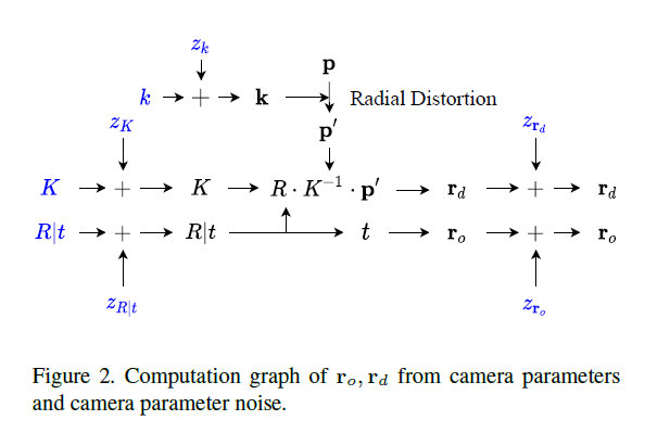
final ray direction, ray offset generation은 Fig.2.에 요약되어 있다.

5. Geometric and Photometric Consistency

우리의 camera model은 camera parameters의 수가 극단적으로 증가하는 generic non-linear distortions을 통합한다. 이 작업에서, 우리는 self-calibration에서 geometric과 photometric consistencies 모두를 사용하는것을 제안한다, consistencies가 additional constraints를 제공하기 때문에 이것은 더 정확한 camera parameter calibration이 가능하게 한다. 이번 섹션에서 우리는 constraints 각각을 discuss해본다.

Geom. Consistency: Projected Ray Distance

generic camera model은 geometric loss를 정의하는 새로운 과제를 제기한다.
대부분의 정통적인 과제에서,
geometric loss는
1) epipolar line과 corresponding한 point간의 distance를 측정하는 epipolar constraint 또는
2) correspondence에 대한 3D point가 정의되고 projection과 correspondence간의 distance를 측정하기 위해 image plane에 projected되는데 이때의 reprojection error에 의해 정의된다.

그러나 이 방법은 우리가 generic noise model을 사용할때 약간의 제약이 있다.

첫째, epipolar distance는 완벽한 pinhole camera를 가정한다, 이것은 우리의 seup을 깨트린다.
둘째, 3D reprojection error는 non-differentiable process를 이용하여 3D point clound reconstruction을 만드는것을 요구하며 camera parameters는 3D reconstruction으로부터 indirectly로 학습된다.

본 작업에서, reprojection error와 같이 indirect loss를 계산하여 3D reconstruction을 요구하는것보다, 우리는 rays간의 discrepancy(차이)를 직접적으로 측정하는 projected ray distance loss를 제안한다.

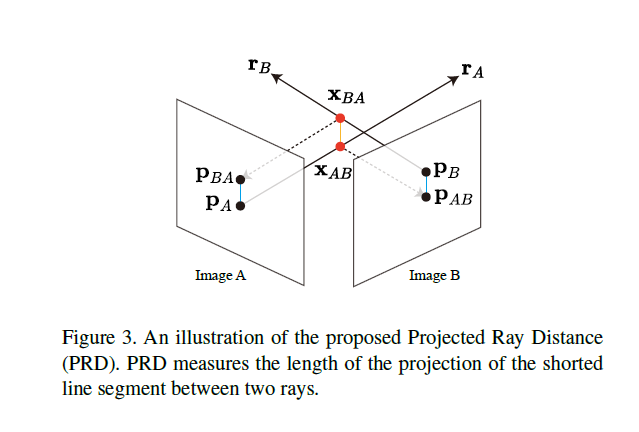
Fig 3 참고 (\(\mathbf{p}_A \leftrightarrow \mathbf{p}_B\))는 camera 1과 camera 2 각각에 correspondence하다고 하자.
모든 camera parameters는 calibrated되었을때, ray \(\mathbf{r}_A\) 와 \(\mathbf{r}_B\)는 point \(\mathbf{p}_A\)와 \(\mathbf{p}_B\)를 만들어 내는 3D point에 교차한다.

그러나, camera parameters에서 error 때문에 misalignment가 생길때, 우리는 corresponding rays간의 가장 짧은 distance를 계산함으로써 deviation(편차)를 측정할 수 있다.

line A위의 point를 \(\mathbf{x}_A(t_A) = \mathbf{r}_{o,A} + t_A\mathbf{r}_{d,A}\) 이고
line B위의 point는 \(\mathbf{x}_B(t_B) = \mathbf{r}_{o,B} + t_B\mathbf{r}_{d,B}\) 라고 하자.

line A와 line B위의 point간의 거리를 다음과 같이 나타낼 수 있다. \[d = \frac{|(\mathbf{r}_{o,B} + t_B\mathbf{r}_{d,B} - \mathbf{r}_{o,A}) \times \mathbf{r}_{A,d}|}{ \mathbf{r}_{A,d} \cdot \mathbf{r}_{A,d}}\]

이것은 \(\hat{t}_B\)에 대해 미분해서 0이 나오는
\(\frac{\mathbf{d}d^2}{\mathbf{d}t_B}\vert_{\hat{t}_B} = 0\) 인 지점에서의 \(\hat{t}_B\)를 구할 수 있다. \[\hat{t}_B = \frac{ (\mathbf{r}_{A,o} - \mathbf{r}_{B,o}) \times \mathbf{r}_{A,d} \cdot (\mathbf{r}_{A,d} \times \mathbf{r}_{B,d})}{(\mathbf{r}_{A,d} \times \mathbf{r}_{B,d})^2}\]

그러면 이 거리를 가장 짧게하는 지점\(\hat{t}_B\)에서의 line B위의 점 \(\hat{\mathbf{x}}_B = \mathbf{x}_B(\hat{t}_B)\)를 얻을 수 있다.

같은 방식으로 \(\mathbf{\hat{x}}_A\)을 얻을 수 있다. 간단하게 하기위해, 우리는 주로 최종 해결책에 초점을 맞출 것이기 때문에, 우리는 \(\mathbf{x}\)를 \(\mathbf{\hat{x}}\)로 표기한다. 2개의 points간의 distanc \(\hat{d} = \bar{\mathbf{x}_A\mathbf{x}_B}\) 는 다음과 같다. \[\hat{d} = \frac{|(\mathbf{r}_{A,o} - \mathbf{r}_{B,o}) \cdot (\mathbf{r}_{A,d} \times \mathbf{r}_{B,d})|}{|\mathbf{r}_{A,d} \times \mathbf{r}_{B,d}|}\]

그러나, 이 distance는 correspondences에 normalized되어 있지않다. 동일한 camera distortions을 고려할 때 카메라에서 멀리 떨어진 지점에 대한 correspondence은 편차(deviation)가 더 큰 반면, 카메라에 더 가까운 지점에 대한 correspondence은 편차(deviation)가 더 작다.

그래서, 우리는 distance의 scale을 normalize할 필요가 있다. 따라서, 우리는 3D space에서 distance를 directly하게 사용하는것보다 , points \(\mathbf{x}_A,\mathbf{x}_B\)를 image planes \(I_A, I_B\)에 project하고 image planes에서 dostance를 계산한다. \[d_{\pi} = \frac{||\pi_A(\mathbf{x}_B) - \mathbf(p)_A || + ||\pi_B(\mathbf{x}_A) - \mathbf(p)_B||}{2}\]

\(\pi(\cdot)\)은 projection function이고 camera와의 distance와 관계없이 각 correspondence의 기여도는 균등하다.

이 projected ray distance는 epipolar distance또는 reprojection error와 다른 novel geometric loss이다. epipolar distance는 오로지 linear pinhole cameras로부터 정의되고 non-linear camera distortions를 modeling 할 수 없다.
다시말해, reprojection error는 non-diffenrentiable preprocessing stage에서 3D reconstruction을 추출하는것을 요구하며 3D reconstruction을 optimizing을 통해 camera parameters를 optimize한다.
우리의 projected ray distance는 intermediate 3D reconstruction을 요구하지 않으며 non-linear camera distortions를 modeling 할 수 있다.

5.2 Chirality Check

camera distortion은 large하고 cameras간 baseline은 작을때, correspondence간의 rays간의 shortest line은 cameras 뒤에 위치하게 될것이다. 이러한 가치없는 ray distance를 최소화하는것은 suboptimal camera parameters를 이끈다. 따라서 우리는 camera rays에 따른 z-depth를 계산함으로써 points가 camera뒤에 있는지 없는지 확인한다. 수식적으로는 다음과 같다. \[R_A \mathbf{x}_B [z] > 0, R_B \mathbf{x}_A [z] > 0\]

\(\mathbf{x}[z]\)는 vector의 z component를 가리킨다.
최종적으로, 우리는 geometric loss를 계산하기 위해 모든 correspondeces에 대해 valid projected ray distances를 평균한다.

Photometric Consistency

geometric consistency와 달리, photometric consistency는 3D geometry를 reconstructing하는것을 요구한다. 왜냐하면 3D point의 color가 현재 perspective에서 visible이 유효한지 아닌지 보기위해서 이다.
우리 작업에서는, 우리는 3D occupancy와 color를 reconstruct하기위해 neural radiance field를 사용한다. 이 implicit representation은 position과 color value를 통해 미분가능하며 volumetric rendering을 통해 visible surface를 capture할 수 있게해준다. 특별히, rendering process 동안, ray는 \(\mathbf{z}_o[\cdot], \mathbf{z}_d[\cdot]\) 뿐만 아니라 \(\Delta K, \Delta a \Delta t\) 뿐만 아니라 \(K_0, R_0, t_0\)를 이용해서 parameterized된다.
우리의 self-calibration model을 optimize하기위해 learnable camera parameters와 관련하여 다음 energy function을 정의한다. \[\mathcal{L} = \sum_{\mathbf{p}\in\mathcal{I}} || C(\mathbf{p}) - \hat{C}(\mathbf{\mathbf{r(p)}}) ||^2_2\]

여기 \(\mathbf{p}\)는 pixel coordinate이고 \(\mathcal{I}\)는 image에서 pixel coordinate의 집합이다.
\(\hat{C}(\mathbf{r})\)은 ray \(\mathbf{r}\)을 이용한 volumetric rendering의 output이고 이것은 pixel \(\mathbf{p}\)에 corresponds하다.
\(C(\mathbf{p})\)는 ground truth color이다. 따라서 intrinsics에 대한 gradient는 다음과 같다. \[\frac{\partial L}{\partial \Delta K} = \frac{\partial L}{\partial \mathbf{r}} (\frac{\partial \mathbf{r}}{\partial \mathbf{r}_d} \frac{\partial \mathbf{r}_d}{\partial \Delta K} + \frac{\partial \mathbf{r}}{\partial \mathbf{r}_o} \frac{\partial \mathbf{r}_o}{\partial \Delta K} + \frac{\partial L}{\partial \mathbf{r}_d} \frac{ \mathbf{r}_d}{\partial \Delta K})\]

비슷하게, 우리는 parameters의 나머지 \(\Delta a, \Delta t\) 뿐만아니라 \(\mathbf{z}_o[\cdot], \mathbf{z}_d[\cdot]\) 그리고 calibration cameras 에 대해서 gradients를 정의할 수 있다.

6. Optimizing Geometry and Camera

geometry와 camera parameters를 optimize하기 위해, 우리는 neural radiance field와 camera model을 jointly하게 learn한다. 그러나, geometry를 모르거나 self-calibration에 대해 너무 coarse하면 정확한 camera parameters를 학습하는것은 불가능하다.
따라서, 우리는 순차적으로 parameters를 learn한다 : geometry와 linear camera model을 먼저 그리고 complex camera model parameters를 다음으로 한다.

6.1 Curriculum learning

camera parameters는 NeRF learning에 대해 rays의 positions와 directions를 결정한다, 그리고 unstable values는 종종 divergence(발산) 또는 sub-optimal results를 낸다. 따라서, 우리는 cameras와 geometry의 learning의 complexity를 jointly하게 줄이기 위해 a subset of learning parameters를 optimization process에 더한다.

먼저, 우리는 camera focal lengths와 focal centers를 image의 width와 height로 초기화를 하면서 NeRF networks를 learn한다. Learning coarse geometry를 처음에 중요하다. 왜냐하면 networks가 더 나은 camera parameters를 학습하기 위한 보다 유리한 local optimum로 네트워크를 초기화하기 때문이다.

다음으로, 우리는 순차적으로 linear camera model, radial distortion, 그리고 ray의 nonlinear noise와 ray origin을 learning에 더해준다. 우리는 overfitting을 줄이고 빠르게 training하기위해 먼저 simpler camera models를 learn한다.

6.2. Joint OPtimization

7. Experiment

7.1 Dataset

7.2 Self-Calibration

우리는 우리의 모델이 camera information을 self-calibrate할 수 있는지를 시연하기위해 밑바닥부터 train하였다.
우리는 모든 rotation matrices, translation vectors 그리고 focal lengths를 indentity matrix와 zero vector, 그리고 captured된 images의 height와 width로 초기화하였다.
Table 1은 training dataset에 대해 rendered된 images의 quality를 보여준다. 비록 우리 모델은 calibrated camera information을 사용하지 않지만, 우리의 모델이 믿을만한 rendering performance를 보여준다.
더욱이 몇몇 scenes에대해, 우리의 model은 COLMAP camera information으로 학습된 NeRF를 능가하였다.