CVPR 2020 paper

39회 인용

• Abstract
• 1. Introduction
• 2. Related Work
• 3. Point-GNN for 3D Object Detection in a Point Cloud
• 3.1. Graph Construction
• 3.2. Graph Neural Network with AutoRegistration
• 3.3. Loss
• 3.4. Box Merging and Scoring
• 4. Experiments
  • 4.1. Dataset
  • 4.2. Implementation Details
  • 4.3. Data Augmentation
  • 4.3.1 Results
  • 4.4. Ablation Study
• 5. Conclusion

Abstract

In this paper, we propose a graph neural network to detect objects from a LiDAR point cloud.
Towards this end, we encode the point cloud efficiently in a fixed radius near-neighbors graph.
We design a graph neural network, named Point-GNN, to predict the category and shape of the object that each vertex in the graph belongs to.

본 논문에서는 LiDAR point cloud에서 개체를 감지하기 위한 graph neural network을 제안한다.
이를 위해, 우리는 고정된 radius near-neighbors graph에서 point cloud를 효율적으로 인코딩한다.
우리는 그래프의 각 정점(vertex)이 속하는 객체의 범주와 모양을 예측하기 위해 Point-GNN이라는 graph neural network을 설계한다.

In Point-GNN, we propose an auto-registration mechanism to reduce translation variance, and also design a box merging and scoring operation to combine detections from multiple vertices accurately.
Our experiments on the KITTI benchmark show the proposed approach achieves leading accuracy using the point cloud alone and can even surpass fusion-based algorithms.
Our results demonstrate the potential of using the graph neural network as a new approach for 3D object detection.

Point-GNN에서는 translation variance을 줄이기 위한 auto-registration mechanism을 제안하고, 여러 정점(multiple vertices)에서 검출된 것을 정확하게 결합하기 위한 상자 병합(box merging) 및 채점 연산(scoring operation)을 설계한다.
KITTI 벤치마크에 대한 우리의 실험은 제안된 접근 방식이 point cloud만을 사용하여 선도적인 정확도를 달성하고 융합 기반 알고리즘도 능가할 수 있음을 보여준다.
우리의 결과는 graph neural network을 3D object detection를 위한 새로운 접근법으로 사용할 가능성을 보여준다.

The code is available at
https://github.com/WeijingShi/Point-GNN

1. Introduction

Understanding the 3D environment is vital in robotic perception.
A point cloud that composes a set of points in space is a widely-used format for 3D sensors such as LiDAR.
Detecting objects accurately from a point cloud is crucial in applications such as autonomous driving.

robotic perception에서는 3D environment을 이해하는 것이 매우 중요하다.
공간의 point 집합을 구성하는 point cloud은 LiDAR과 같은 3D 센서에 널리 사용되는 형식이다.
point cloud에서 물체를 정확하게 감지하는 것은 자율 주행과 같은 애플리케이션에서 중요하다.

Convolutional neural networks that detect objects from images rely on the convolution operation.
While the convolution operation is efficient, it requires a regular grid as input.
Unlike an image, a point cloud is typically sparse and not spaced evenly on a regular grid.
Placing a point cloud on a regular grid generates an uneven number of points in the grid cells.
Applying the same convolution operation on such a grid leads to potential information loss in the crowded cells or wasted computation in the empty cells.

이미지에서 물체를 감지하는 Convolutional neural networks은 convolution operation에 의존한다.
convolution operation은 효율적이지만 입력으로 정규 그리드가 필요하다.
이미지와 달리, point cloud은 일반적으로 sparse하고 정규 그리드에 고르게 분포되어 있지 않는다.
point cloud을 일반 그리드에 배치하면 그리드 셀에서 불균일한 수의 point가 생성된다.
그러한 그리드에 동일한 convolution 연산을 적용하면 crowded cells에서 잠재적 정보 손실(potential information loss) 또는 빈 셀에서 낭비되는 계산으로 이어진다.

Recent breakthroughs in using neural networks [3] [22] allow an unordered set of points as input.
Studies take advantage of this type of neural network to extract point cloud features without mapping the point cloud to a grid.
However, they typically need to sample and group points iteratively to create a point set representation.
The repeated grouping and sampling on a large point cloud can be computationally costly.
Recent 3D detection approaches [10] [21] [16] often take a hybrid approach to use a grid and a set representation in different stages.
Although they show some promising results, such hybrid strategies may suffer the shortcomings of both representations.

신경망을 사용하는 최근의 발전[3] [22]은 정렬되지 않은 points 집합을 입력으로 허용한다.
연구는 이러한 유형의 neural network을 활용하여 point cloud를 그리드에 매핑하지 않고 point cloud features을 추출한다.
그러나 일반적으로 point set representation을 만들려면 point을 반복적으로 sampling하고 grouping해야 한다.
large point cloud에서 반복된 grouping 및 sampling은 계산 비용이 많이 들 수 있다.
최근의 3D 감지 접근법[10] [21] [16]은 종종 다른 단계에서 grid 및 set representation을 사용하기 위해 hybrid 접근법을 채택한다.
비록 몇 가지 유망한 결과를 보여주지만, 그러한 hybrid 전략은 두 가지 표현의 단점을 겪을 수 있다.

In this work, we propose to use a graph as a compact representation of a point cloud and design a graph neural network called Point-GNN to detect objects.
We encode the point cloud natively in a graph by using the points as the graph vertices.
The edges of the graph connect neighborhood points that lie within a fixed radius, which allows feature information to flow between neighbors.
Such a graph representation adapts to the structure of a point cloud directly without the need to make it regular.
A graph neural network reuses the graph edges in every layer, and avoids grouping and sampling the points repeatedly.

본 연구에서는 graph를 point cloud의 compact representation으로 사용하고 객체를 감지하기 위해 Point-GNN이라는 graph neural network 설계를 제안한다.
우리는 point을 graph vertices으로 사용하여 graph에서 point cloud을 기본적으로 인코딩한다.
graph의 edges는 고정 반지름 내에 있는 neighborhood points을 연결하므로, 인접 영역 간에 feature information가 흐를 수 있다.
이러한 graph representation은 정기적으로 설정할 필요 없이 포인트 클라우드의 구조에 직접 적응한다.
graph neural network은 모든 layer에서 graph edges를 재사용하고 점의 grouping 및 sampling을 반복적으로 추출하지 않는다.

Studies [15] [9] [2] [17] have looked into using graph neural network for the classification and the semantic segmentation of a point cloud.
However, little research has looked into using a graph neural network for the 3D object detection in a point cloud.
Our work demonstrates the feasibility of using a GNN for highly accurate object detection in a point cloud.

연구[15] [9] [2] [17]은 point cloud의 classification 및 semantic segmentation을 위해 graph neural network 사용을 조사했다.
그러나 point cloud에서 3D object detection를 위한 graph neural network 사용에 대한 연구는 거의 없었다.
우리의 연구는 point cloud에서 매우 정확한 객체 탐지를 위해 GNN을 사용할 가능성을 보여준다.

Our proposed graph neural network Point-GNN takes the point graph as its input.
It outputs the category and bounding boxes of the objects to which each vertex belongs.
Point-GNN is a one-stage detection method that detects multiple objects in a single shot.
To reduce the translation variance in a graph neural network, we introduce an auto-registration mechanism which allows points to align their coordinates based on their features.
We further design a box merging and scoring operation to combine detection results from multiple vertices accurately.

제안된 graph neural network Point-GNN은 point graph를 입력으로 삼는다.
각 vertex이 속하는 객체의 category 및 bounding boxes를 출력한다.
Point-GNN은 single shot으로 여러 개체를 감지하는 one-stage detection method이다.
graph neural network의 변환 분산(translation variance)을 줄이기 위해, 우리는 점들이 특징에 따라 좌표를 align(정렬)할 수 있는 auto-registration mechanism을 도입한다.
우리는 여러 vertex에서 검출 결과를 정확하게 결합하기 위해 box merging 및 scoring operation을 추가로 설계한다.

We evaluate the proposed method on the KITTI benchmark.
On the KITTI benchmark, Point-GNN achieves the state-of-the-art accuracy using the point cloud alone and even surpasses sensor fusion approaches.
Our Point-GNN shows the potential of a new type 3D object detection approach using graph neural network, and it can serve as a strong baseline for the future research.
We conduct an extensive ablation study on the effectiveness of the components in Point-GNN.

제안된 방법을 KITTI 벤치마크에서 평가한다.
KITTI 벤치마크에서 Point-GNN은 point cloud만을 사용하여 state-of-the-art accuracy를 달성하고 센서 융합 접근 방식까지 능가한다.
우리의 Point-GNN은 graph neural network을 이용한 새로운 유형의 3D 객체 감지 접근법의 잠재력을 보여주며, 향후 연구를 위한 강력한 baseline으로 작용할 수 있다.
우리는 Point-GNN에서 components의 효과에 대한 광범위한 절제 연구를 수행한다.

In summery, the contributions of this paper are:

• We propose a new object detection approach using graph neural network on the point cloud.
• We design Point-GNN, a graph neural network with an auto-registration mechanism that detects multiple objects in a single shot.
• We achieve state-of-the-art 3D object detection accuracy in the KITTI benchmark and analyze the effectiveness of each component in depth.

• point cloud에서 graph neural network을 이용한 새로운 객체 감지 접근 방식을 제안한다.
• 우리는 single shot으로 여러 개체를 감지하는 auto-registration mechanism이 있는 graph neural network Point-GNN을 설계한다.
• KITTI 벤치마크에서 state-of-the-art 3D object detection accuracy를 달성하고 depth에서 각 component의 효과를 분석한다.

2. Related Work

Prior work in this context can be grouped into three categories, as shown in Figure 1.

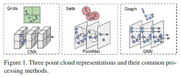
Point cloud in grids.
Many recent studies convert a point cloud to a regular grid to utilize convolutional neural networks.
[20] projects a point cloud to a 2D Bird’s Eye View (BEV) image and uses a 2D CNN for object detection.
[4] projects a point cloud to both a BEV image and a Front View (FV) image before applying a 2D CNN on both.
Such projection induces a quantization error due to the limited image resolution.
Some approaches keep a point cloud in 3D coordinates.
[23] represents points in 3D voxels and applies 3D convolution for object detection.
When the resolution of the voxels grows, the computation cost of 3D CNN grows cubically, but many voxels are empty due to point sparsity.
Optimizations such as the sparse convolution [19] reduce the computation cost.
Converting a point cloud to a 2D/3D grid suffers from the mismatch between the irregular distribution of points and the regular structure of the grids.

최근의 많은 연구는 point cloud를 regular grid로 변환하여 convolutional neural networks을 활용한다.
[20] point cloud를 2D BEV(Bird’s Eye View) image에 투영하고 object detection을 위해 2D CNN을 사용한다.
[4]은 BEV image와 FV(Front View) image에 point cloud을 투영한 후 두 image 모두에 2D CNN을 적용한다.
이러한 투영은 제한된 image resolution로 인해 quantization error를 유도한다.
일부 접근 방식은 point cloud를 3D 좌표로 유지한다.
[23]은 3D voxels의 점을 나타내며 object detection를 위해 3D convolution을 적용한다.
voxels의 해상도가 증가하면 3D CNN의 계산 비용은 입체적으로 증가하지만 많은 voxels은 point sparsity으로 인해 비어 있다.
sparse convolution과 같은 Optimizations[19]는 계산 비용을 절감한다.
point cloud를 2D/3D grid로 변환하면 points의 불규칙한 분포(irregular distribution)와 grids의 규칙적인 구조(regular structure) 사이의 불일치가 발생한다.

Point cloud in sets.
Deep learning techniques on sets such as PointNet [3] and DeepSet[22] show neural networks can extract features from an unordered set of points directly.
In such a method, each point is processed by a multi-layer perceptron (MLP) to obtain a point feature vector.
Those features are aggregated by an average or max pooling function to form a global feature vector of the whole set.
[14] further proposes the hierarchical aggregation of point features, and generates local subsets of points by sampling around some key points.
The features of those subsets are then again grouped into sets for further feature extraction.
Many 3D object detection approaches take advantage of such neural networks to process a point cloud without mapping it to a grid.
However, the sampling and grouping of points on a large scale lead to additional computational costs.
Most object detection studies only use the neural network on sets as a part of the pipeline.
[13] generates object proposals from camera images and uses [14] to separate points that belong to an object from the background and predict a bounding box.
[16] uses [14] as a backbone network to generate bounding box proposals directly from a point cloud.
Then, it uses a second-stage point network to refine the bounding boxes.
Hybrid approaches such as [23] [19] [10] [21] use [3] to extract features from local point sets and place the features on a regular grid for the convolutional operation.
Although they reduce the local irregularity of the point cloud to some degree, they still suffer the mismatch between a regular grid and the overall point cloud structure.

PointNet [3] 및 DeepSet[22]와 같은 sets에 대한 딥 러닝 기술은 신경망이 unordered set of points에서 직접 features을 추출할 수 있음을 보여준다.
이러한 방법에서 각 point은 point feature vector를 얻기 위해 multi-layer perceptron (MLP)에 의해 처리된다.
이러한 features은 average 또는 max pooling function에 의해 집계되어 전체 집합의 global feature vector를 형성한다.
[14] point features의 계층적 집계(hierarchical aggregation)를 추가로 제안하고, 일부 key points들을 sampling하여 points의 local subsets을 생성한다.
그런 다음 subsets의 features은 추가 feature 추출을 위해 sets로 다시 grouping된다.
많은 3D object detection 접근 방식은 이러한 신경망을 이용하여 grid에 매핑하지 않고 point cloud를 처리한다.
그러나 large scale로 points을 sampling하고 grouping하면 추가 계산 비용이 발생한다.
대부분의 object detection 연구는 sets에 신경망만 pipeline의 일부로 사용한다.
‘Frustum Point’은 camera images에서 object proposals을 생성하고 PointNet++를 사용하여 개체에 속한 points을 배경에서 분리하고 bounding box를 예측한다.
‘Point-RCNN’은 PointNet++를 backbone network로 사용하여 point cloud에서 직접 bounding box proposals을 생성합니다.
그런 다음, 2단계 point network를 사용하여 bounding boxes를 세분화한다.
[23] [19] [10] [21]과 같은 Hybrid 접근 방식은 [3]을 사용하여 local point sets에서 features을 추출하고 convolutional operation을 위해 regular grid에 features을 배치한다.
point cloud의 local irregularity은 어느 정도 감소하지만, 여전히 regular grid와 overall point cloud structure간의 불일치를 겪는다.

Point cloud in graphs.
Research on graph neural network [18] seeks to generalize the convolutional neural network to a graph representation.
A GNN iteratively updates its vertex features by aggregating features along the edges.
Although the aggregation scheme sometimes is similar to that in deep learning on sets, a GNN allows more complex features to be determined along the edges.
It typically does not need to sample and group vertices repeatedly.
In the computer vision domain, a few approaches represent the point cloud as a graph.
[15] uses a recurrent GNN for the semantic segmentation on RGBD data.
[9] partitions a point cloud to simple geometrical shapes and link them into a graph for semantic segmentation.
[2] [17] look into classifying a point cloud using a GNN.
So far, few investigations have looked into designing a graph neural network for object detection, where an explicit prediction of the object shape is required.

graph neural network[18]에 대한 연구는 convolutional neural network을 graph representation으로 generalize하려고 한다.
GNN은 edges(간선)를 따라 features을 집계하여 vertex(정점) features을 반복적으로 업데이트한다.
aggregation scheme가 때때로 sets에 대한 deep learning에서와 유사하지만, GNN을 사용하면 edges를 따라 더 complex features을 결정할 수 있다.
일반적으로 vertices을 반복적으로 샘플링하고 그룹화할 필요가 없다.
computer vision 도메인에서 몇 가지 접근 방식은 point cloud를 graph로 나타낸다.
[15]는 RGBD data의 semantic segmentation을 위해 반복 GNN을 사용한다.
[9] point cloud을 단순한 geometrical shapes에 분할하고 이를 semantic segmentation을 위한 graph로 link한다.
[2] [17] GNN을 사용하여 point cloud를 분류합니다.
지금까지 object shape의 명시적 예측이 필요한 object detection를 위한 graph neural network 설계를 검토한 연구는 거의 없다.

Our work differs from previous work by designing a GNN for object detection.
Instead of converting a point cloud to a regular gird, such as an image or a voxel, we use a graph representation to preserve the irregularity of a point cloud.
Unlike the techniques that sample and group the points into sets repeatedly, we construct the graph once.
The proposed Point-GNN then extracts features of the point cloud by iteratively updating vertex features on the same graph.
Our work is a single-stage detection method without the need to develop a second-stage refinement neural networks like those in [4][16][21][11][13].

우리의 작업은 object detection를 위한 GNN을 설계함으로써 이전 작업과 다르다.
point cloud를 image 또는 voxel과 같은 regular gird로 변환하는 대신 graph representation을 사용하여 point cloud의 불규칙성(irregularity)을 보존한다.
points을 반복적으로 샘플링하고 세트로 그룹화하는 기술과 달리, 우리는 graph를 한 번 구성한다.
그런 다음 제안된 Point-GNN은 동일한 graph에 vertex features을 반복적으로 업데이트하여 point cloud의 features을 추출한다.
우리의 연구는 [4][16][21][11][13]과 같은 second-stage refinement neural networks을 개발할 필요가 없는 single-stage detection method이다.

3. Point-GNN for 3D Object Detection in a Point Cloud

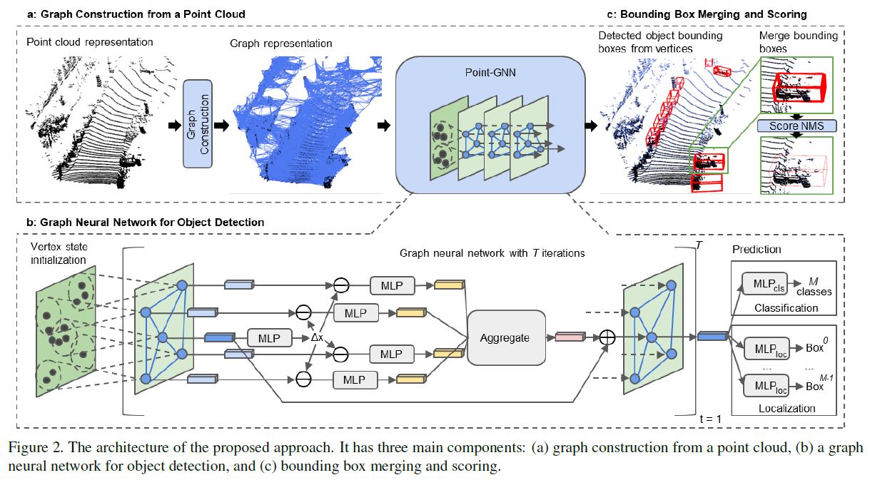
In this section, we describe the proposed approach to detect 3D objects from a point cloud.
As shown in Figure 2, the overall architecture of our method contains three components:
(a) graph construction, (b) a GNN of T iterations, and (c) bounding box merging and scoring.

3.1. Graph Construction

Formally, we define a point cloud of \(N\) points as a set \(P = \{p_1, ... , p_N\}\), where \(p_i = (x_i, s_i)\) is a point with both 3D coordinates \(x_i \in R^3\) and the state value \(s_i \in R^k\) a \(k\)-length vector that represents the point property.
The state value \(s_i\) can be the reflected laser intensity or the features which encode the surrounding objects.
Given a point cloud \(P\), we construct a graph \(G = (P,E)\) by using \(P\) as the vertices and connecting a point to its neighbors within a fixed radius \(r\), i.e. \[E = \{(p_i, p_j) | \; ||x_i - x_j||_2 < r\} \qquad \qquad \qquad (1)\]

The construction of such a graph is the well-known fixed radius near-neighbors search problem.
By using a cell list to find point pairs that are within a given cut-off distance, we can efficiently solve the problem with a runtime complexity of \(O(cN)\) where \(c\) is the max number of neighbors within the radius [1].

이러한 graph의 구성은 near-neighbors search problem에서 잘 알려진 fixed radius이다.
cell list을 사용하여 주어진 cut-off distance 내에 있는 point pairs을 찾아냄으로써, 우리는 \(c\)가 반지름 내 최대 neighbors 수인 \(O(cN)\)의 runtime 복잡성으로 문제를 효율적으로 해결할 수 있다[1].

a set \(P = \{p_1, ... , p_N\}\) : \(N\) Points의 point cloud
\(p_i = (x_i, s_i)\) : a point with both 3D coordinates \(x_i \in R^3\)
state value \(s_i \in R^k\) a \(k\)-length vector
state value \(s_i\) : reflected laser intensity
\(k\)-length vector : point property를 표현
graph \(G\) : \(G = (P,E)\), P : point cloud set이자 vertices
edges \(E\) : \(E = \{(p_i, p_j) | \; ||x_i - x_j||_2 < r\}\)
r : fixed radius
c : max number of neighbors within the radius
O() : big-O 표기법, 공간 복잡성, 시간 복잡성

In practice, a point cloud commonly comprises tens of thousands of points.
Constructing a graph with all the points as vertices imposes a substantial computational burden.
Therefore, we use a voxel downsampled point cloud \(\hat{P}\) for the graph construction.
It must be noted that the voxels here are only used to reduce the density of a point cloud and they are not used as the representation of the point cloud.
We still use a graph to present the downsampled point cloud.

실제로 point cloud는 일반적으로 수만 개의 points로 구성된다.
모든 점을 vertices으로 하여 graph를 구성하면 상당한 계산 부담이 발생한다.
따라서 우리는 graph construction을 위해 voxel downsampled point cloud \(\hat{P}\)를 사용한다.
여기서 voxels은 point cloud의 density를 줄이는 데만 사용되며 point cloud의 표현으로 사용되지 않는다는 점에 유의해야 한다.
우리는 여전히 그래프를 사용하여 다운샘플링된 point cloud을 제시한다.

To preserve the information within the original point cloud, we encode the dense point cloud in the initial state value \(s_i\) of the vertex.
More specifically, we search the raw points within a \(r_0\) radius of each vertex and use the neural network on sets to extract their features.
We follow [10] [23] and embed the lidar reflection intensity and the relative coordinates using an \(MLP\) and then aggregate them by the \(Max\) function.
We use the resulting features as the initial state value of the vertex.
After the graph construction, we process the graph with a GNN, as shown in Figure 2b.

original point cloud의 정보를 보존하기 위해 vertex의 initial state value \(s_i\)에서 dense point cloud를 인코딩한다.
보다 구체적으로, 우리는 각 vertex의 \(r_0\) radius 내에서 raw points를 검색하고 집합에 신경망을 사용하여 features을 추출한다.
우리는 [10] [23]을 따르고 \(MLP\)를 사용하여 lidar reflection intensity와 relative coordinates를 embed한 다음 \(Max\) function으로 그것들을 집계한다.
우리는 결과 features을 vertex의 initial state value으로 사용한다.
graph construction 후 Figure 2b와 같이 GNN을 사용하여 graph를 처리한다.

3.2. Graph Neural Network with AutoRegistration

A typical graph neural network refines the vertex features by aggregating features along the edges.
In the \((t+1)^{th}\) iteration, it updates each vertex feature in the form:

\(v^{t+1}_i = g^t(p(\{e_{ij}^t | (i, j) \in E\}), v^t_i )\)
\(e_{ij}^t= f^t(v^t_i , v^t_j)\)

where \(e^t\) and \(v^t\) are the edge and vertex features from the \(t^{th}\) iteration.
A function \(f^t(.)\) computes the edge feature between two vertices.
\(p(.)\) is a set function which aggregates the edge features for each vertex.
\(g^t(.)\) takes the aggregated edge features to update the vertex features.
The graph neural network then outputs the vertex features or repeats the process in the next iteration.

\(e^t\) : edge features from the \(t^{th}\) iteration
\(v^t\) : vertex features from the \(t^{th}\) iteration
fuction \(f^t(.)\) : 두 vertices간의 edge feature 계산
\(p(.)\) : a set function which aggregates the edge features for each vertex
\(g^t(.)\) : the aggregated edge features to update the vertex features

In the case of object detection, we design the GNN to refine a vertex’s state to include information about the object where the vertex belongs.

object detection의 경우, 우리는 vertex이 속하는 객체에 대한 정보를 포함하도록 vertex의 상태를 정제하도록 GNN을 설계한다.

Towards this goal, we re-write Equation (2) to refine a vertex’s state using its neighbors’ states: \[s^{t+1}_i = g^t(p(\{f^t(x_j - x_i, s^t_j) | (i, j) \in E\}), s^t_i ) \qquad \qquad \qquad (3)\]

Note that we use the relative coordinates of the neighbors as input to \(f^t(.)\) for the edge feature extraction.
The relative coordinates induce translation invariance against the global shift of the point cloud.

우리는 edge feature extraction을 위해 \(f^t(.)\)에 대한 입력으로 neighbors의 상대 좌표(relative coordinates)를 사용한다.
상대 좌표는 point cloud의 global shift에 대한 변환 불변성(translation invariance)을 유도한다.

However, it is still sensitive to translation within the neighborhood area.
When a small translation is added to a vertex, the local structure of its neighbors remains similar.
But the relative coordinates of the neighbors are all changed, which increases the input variance to \(f^t(.)\).
To reduce the translation variance, we propose aligning neighbors’ coordinates by their structural features instead of the center vertex coordinates.
Because the center vertex already contains some structural features from the previous iteration, we can use it to predict an alignment offset, and propose an auto-registration mechanism:

하지만, 그것은 여전히 neighborhood area 내에서의 translation에 민감하다.
작은 translation이 vertex에 추가될 때, neighbors의 local structure는 비슷하게 유지된다.
그러나 neighbors의 상대 좌표가 모두 변경되어 입력 분산(input variance)이 \(f^t(.)\)로 증가한다.
변환 분산(translation variance)을 줄이기 위해, 우리는 중심 정점(center vertex) 좌표 대신 structural features으로 neighbors의 좌표를 aligning하는 것을 제안한다.
center vertex는 이미 이전 반복의 일부 structural features을 포함하고 있기 때문에 이를 사용하여 alignment offset을 예측하고 auto-registration mechanism을 제안할 수 있다:

\(\Delta x_i^t = h^t(s^t_i) \qquad \qquad \qquad (4)\)
\(s^{t+1}_i = g^t(p({f(x_j - x_i + \Delta x_i^t, s^t_j)}, s^t_i)\)

\(\Delta x_i^t\) is the coordination offset for the vertices to register their coordinates.
\(h^t(.)\) calculates the offset using the center vertex state value from the previous iteration.
By setting \(h^t(.)\) to output zero, the GNN can disable the offset if necessary.
In that case, the GNN returns to Equation (3).
We analyze the effectiveness of this auto-registration mechanism in Section 4.

\(\Delta x_i^t\)는 vertex들이 좌표를 등록하기 위한 조정 offset이다.
\(h^t(.)\)는 이전 iteration의 center vertex state value을 사용하여 offset을 계산한다.
\(h^t(.)\)를 output zero으로 설정하여 GNN은 필요한 경우 offset을 비활성화할 수 있다.
이 경우 GNN은 Equation (3)으로 돌아간다. 우리는 Section 4에서 auto-registration mechanism의 효과를 분석한다.

As shown in Figure 2b, we model \(f^t(.)\), \(g^t(.)\) and \(h^t(.)\) using multi-layer perceptrons (MLP) and add a residual connection in \(g^t(.)\).
We choose \(p(.)\) to be \(Max\) for its robustness[3].
A single iteration in the proposed graph network is then given by:

\(\Delta x_i^t = MLP^t_h(s^t_i)\) \(e^t_{ij} = MLP^t_f([x_j - x_i + \Delta x_i^t, s^t_j])\) \(s^{t+1}_i = MLP^t_g(Max(\{e_{ij} | (i, j) \in E\})) + s^t_i \qquad \qquad \qquad (5)\) where [,] represents the concatenation operation.

Every iteration \(t\) uses a different set of \(MLP^t\), which is not shared among iterations.
After \(T\) iterations of the graph neural network, we use the vertex state value to predict both the category and the bounding box of the object where the vertex belongs.
A classification branch \(MLP_{cls}\) computes a multi-class probability.
Finally, a localization branch \(MLP_{loc}\) computes a bounding box for each class.

모든 iteration \(t\)는 다른 \(MLP^t\) 집합을 사용하며, 이는 iterations 간에 공유되지 않는다.
graph neural network의 \(T\) iterations 후, 우리는 vertex state value을 사용하여 vertex이 속하는 객체의 category와 bounding box를 모두 예측한다.
classification branch \(MLP_{cls}\)는 multi-class probability을 계산한다.
마지막으로, localization branch \(MLP_{loc}\)는 각 class에 대한 bounding box를 계산한다.

3.3. Loss

For the object category, the classification branch computes a multi-class probability distribution \((p_{c_1} , ... , p_{c_M})\) for each vertex.
\(M\) is the total number of object classes, including the Background class.
If a vertex is within a bounding box of an object, we assign the object class to the vertex.
If a vertex is outside any bounding boxes, we assign the background class to it.
We use the average cross-entropy loss as the classification loss. \[l_{cls} = - \frac{1}{N} \sum_{i=1}^N \sum_{j=1}^N y^i_{c_j}log(p^i_{c_j}) \qquad \qquad \qquad (6)\]

,where \(p^i_c\) and \(y^i_c\) are the predicted probability and the one-hot class label for the \(i\)-th vertex respectively.

object category의 경우, classification branch는 각 vertex에 대한 multi-class probability distribution \((p_{c_1} , ... , p_{c_M})\)를 계산한다.
\(M\)은 Background class를 포함한 object classes의 총 수 이다.
vertex이 object의 bounding box 내에 있으면 object class를 vertex에 할당한다.
vertex이 bounding box 외부에 있는 경우 background class를 여기에 할당한다.
우리는 average cross-entropy loss을 classification loss로 사용한다.

For the object bounding box, we predict it in the 7 degree-of-freedom format \(b = (x, y, z, l, h, w, \mathit{\theta})\), where \((x, y, z)\) represent the center position of the bounding box, \((l,h,w)\) represent the box length, height and width respectively, and \(\theta\) is the yaw angle.

We encode the bounding box with the vertex coordinates \((x_v, y_v, z_v)\) as follows:

\(\delta_x = \frac{x-x_v}{l_m},\delta_y = \frac{y-y_v}{h_m},\delta_z = \frac{z-z_v}{w_m}\)
\(\delta_l =log(\frac{l}{l_m}), \delta_h = log(\frac{h}{h_m}), \delta_w = log(\frac{w}{w_m})\)
\(\delta_\theta = \frac{\theta - \theta_0}{\theta_m} \qquad \qquad \qquad (7)\)

,where \(l_m, h_m, w_m, \theta_0, \theta_m\) are constant scale factors.

The localization branch predicts the encoded bounding box \(\delta_b = (\delta_x, \delta_y, \delta_z, \delta_l, \delta_h, \delta_w, \delta_\theta)\) for each class.
If a vertex is within a bounding box, we compute the Huber loss [7] between the ground truth and our prediction.
If a vertex is outside any bounding boxes or it belongs to a class that we do not need to localize, we set its localization loss as zero.
We then average the localization loss of all the vertices: \[l_{loc} = \frac{1}{N} \sum^X_{i=1} \mathbb{1}(v_i \in b_{interest}) \sum_{\delta \in \delta_{b_i}}l_{huber}(\delta - \delta^{gt})\qquad \qquad \qquad (8)\]

To prevent over-fitting, we add L1 regularization to each MLP.
The total loss is then: \(l_{total} =\alpha l_{cls} + \beta l_{loc} + \gamma l_{reg} \qquad \qquad \qquad (9)\)

,where \(\alpha, \beta\) and \(\gamma\) are constant weights to balance each loss.

3.4. Box Merging and Scoring

As multiple vertices can be on the same object, the neural network can output multiple bounding boxes of the same object.
It is necessary to merge these bounding boxes into one and also assign a confidence score.
Non-maximum suppression (NMS) has been widely used for this purpose.
The common practice is to select the box with the highest classification score and suppress the other overlapping boxes.
However, the classification score does not always reflect the localization quality.
Notably, a partially occluded object can have a strong clue indicating the type of the object but lacks enough shape information.
The standard NMS can pick an inaccurate bounding box base on the classification score alone.

multiple vertices이 동일한 객체에 있을 수 있으므로 신경망은 동일한 객체의 여러 bounding boxes를 출력할 수 있다.
이러한 bounding boxes를 하나로 병합하고 confidence score를 할당해야 한다.
Non-maximum suppression (NMS)는 이러한 목적으로 널리 사용되어 왔다.
classification score가 가장 높은 box를 선택하고 겹치는 다른 boxes를 표시하지 않는 것이 일반적이다.
그러나 classification score가 항상 localization quality을 반영하는 것은 아니다.
특히 occluded object는 object의 type을 나타내는 강력한 단서를 가질 수 있지만 충분한 shape information이 부족하다. 표준 NMS는 classification score만으로는 부정확한 bounding box를 선택할 수 있다.

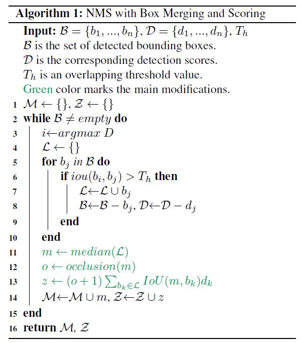
To improve the localization accuracy, we propose to calculate the merged box by considering the entire overlapped box cluster.
More specifically, we consider the median position and size of the overlapped bounding boxes.
We also compute the confidence score as the sum of the classification scores weighted by the Intersection-of-Union (IoU) factor and an occlusion factor.
The occlusion factor represents the occupied volume ratio.
Given a box \(b_i\), let \(l_i, w_i, h_i\) be its length, width and height, and let \(v^l_i, v^w_i , v^h_i\) be the unit vectors that indicate their directions respectively.
\(x_j\) are the coordinates of point \(p_j\).
The occlusion factor \(o_i\) is then:

localization accuracy를 높이기 위해 전체 overlapped box cluster를 고려하여 merged box를 계산할 것을 제안한다.
보다 구체적으로, 우리는 overlapped bounding boxes position와 size를 고려한다.
또한 confidence score를 IOU(Intersection-of-Union) factor와 occlusion factor로 weighted된 classification scores의 합으로 계산한다.
occlusion factor는 점유 volume ratio을 나타낸다.
상자 \(b_i\)가 주어지면 \(l_i, w_i, h_i\)를 길이, 너비 및 높이로 하고 \(v^l_i, v^w_i\)를 각각 방향을 나타내는 단위 벡터(unit vectors)로 한다.
\(x_j\)는 점 \(p_j\)의 좌표이다.
그런 다음 occlusion factor \(o_i\)는 다음과 같다:

\[o_i = \frac{1}{1_i w_i h_i} \prod_{v \in \{v^l_i,v^w_i,v^h_i\}} \max_{p_j \in b_i}(v^T x_j) - \min_{p_j \in b_i}(v^T x_j)\]

We modify standard NMS as shown in Algorithm 1.
It returns the merged bounding boxes \(\mathcal{M}\) and their confidence score \(\mathcal{Z}\).
We will study its effectiveness in Section 4.

4. Experiments

4.1. Dataset

We evaluate our design using the widely used KITTI object detection benchmark [6].
The KITTI dataset contains 7481 training samples and 7518 testing samples.
Each sample provides both the point cloud and the camera image.
We only use the point cloud in our approach.
Since the dataset only annotates objects that are visible within the image, we process the point cloud only within the field of view of the image.
The KITTI benchmark evaluates the average precision (AP) of three types of objects: Car, Pedestrian and Cyclist.
Due to the scale difference, we follow the common practice [10] [23] [19] [21] and train one network for the Car and another network for the Pedestrian and Cyclist.
For training, we remove samples that do not contain objects of interest.

널리 사용되는 KITTI object detection benchmark [6]를 사용하여 설계를 평가한다.
KITTI datase에는 7481개의 training 샘플과 7518개의 testing 샘플이 포함되어 있다.
각 샘플은 point cloud과 camera image를 모두 제공한다.
본 논문은 point cloud만 접근 방식에 사용합니다.
dataset는 이미지 내에서 보이는 objects에만 주석을 달기 때문에, 우리는 이미지의 시야 내에서만 point cloud를 처리한다.
KITTI benchmark는 자동차, 보행자 및 사이클리스트의 세 가지 유형의 average precision(AP)를 평가한다.
scale 차이로 인해, 우리는 일반적인 관례를 따르고 [10] [23] [19] [21], one network for the Car와 another network for the Pedestrian and Cyclist를 훈련시킨다.
training을 위해 관심 개체가 포함되지 않은 샘플을 제거합니다.

4.2. Implementation Details

We use three iterations (T = 3) in our graph neural network.
During training, we limit the maximum number of input edges per vertex to 256.
During inference, we use all the input edges.
All GNN layers perform auto-registration using a two-layer \(MLP_h\) of units (64, 3).
The \(MLP_{cls}\) is of size (64, #(classes)).
For each class, \(MLP_{loc}\) is of size (64, 64, 7).

우리는 그래프 신경망에서 세 번 iterations(T = 3)을 사용한다.
training 동안에, 우리는 vertex당 최대 input edges 수를 256개로 제한한다.
inference 동안에, 우리는 모든 input edges를 사용한다.
모든 GNN layers은 2 layer \(MLP_h\) units (64, 3)를 사용하여 auto-registration을 수행한다.
\(MLP_{cls}\)의 size는 (64, #(classes)).
각 class의 \(MLP_{loc}\) size는 (64, 64, 7).

Car: We set \((l_m, h_m, w_m)\) to the median size of Car bounding boxes (3.88m, 1.5m, 1.63m).
We treat a side-view car with \(\theta \in [-\pi/4, \pi/4]\) and a front-view car \(\theta \in [\pi/4, 3\pi/4]\) as two different classes.
Therefore, we set \(\theta_0 = 0\) and \(\theta_0 = \pi/2\) respectively.
The scale \(\theta_m\) is set as \(\pi/2\).
Together with the Background class and DoNotCare class, 4 classes are predicted.
We construct the graph with \(r = 4m\) and \(r_0 = 1m\).
We set \(\hat{P}\) as a downsampled point cloud by a voxel size of 0.8 meters in training and 0.4 meters in inference.
\(MLP_f\) and \(MLP_g\), are both of sizes (300, 300).
For the initial vertex state, we use an \(MLP\) of \((32, 64, 128, 300)\) for embedding raw points and another \(MLP\) of \((300, 300)\) after the Max aggregation.
We set \(T_h = 0.01\) in NMS.

\((l_m, h_m, w_m)\)를 Car bounding boxes의 중간 크기 자동차 (3.88m, 1.5m, 1.63m)로 설정했다.
우리는 \(\theta \in [-\pi/4, \pi/4]\)가 있는 side-view car와 front-view car \(\theta \in [\pi/4, 3\pi/4]\)을 두 가지 다른 클래스로 취급한다.
\(\theta_0 = 0\)
\(\theta_0 = \pi/2\)로 설정
scale \(\theta_m\) : \(\pi/2\)로 설정
Background 클래스 및 DoNotCare 클래스와 함께 4개의 클래스가 예측된다.
\(r = 4m\) 및 \(r_0 = 1m\)로 graph를 구성한다.
training에서 0.8m의 voxel size로 downsample된 point cloud를 \(\hat{P}\)으로 설정.
inference에서 0.4m의 voxel size로 downsample된 point cloud를 \(\hat{P}\)으로 설정.
\(MLP_f\)와 \(MLP_g\)는 둘 다 size가 (300,300)이다.
initial vertex state의 경우, raw points을 embedding하기 위해 \((32, 64, 128, 300)\)의 \(MLP\)와 \((300, 300)\)의 또 다른 \(MLP\)를 사용한다, Max aggregation 이후에.
우리는 \(T_h = 0.01\)를 NMS로 설정했다.

Pedestrian and Cyclist.
Again, we set \((l_m, h_m, w_m)\) to the median bounding box size.
We set \((0.88m, 1.77m, 0.65m)\) for Pedestrian and \((1.76m, 1.75m, 0.6m)\) for Cyclist.
Similar to what we did with the Car class, we treat front-view and side-view objects as two different classes.
Together with the Background class and the DoNotCare class, 6 classes are predicted.
We build the graph using \(r = 1.6m\), and downsample the point cloud by a voxel size of 0.4 meters in training and 0.2 meters in inference.
\(MLP_f\) and \(MLP_g\) are both of sizes \((256, 256)\).
For the vertex state initialization, we set \(r_0 = 0.4m\).
We use a an MLP of (32, 64, 128, 256, 512) for embedding and an MLP of (256, 256) to process the aggregated feature.
We set \(T_h = 0.2\) in NMS.

다시 \((l_m, h_m, w_m)\)를 median bounding box size로 설정한다.
우리는 보행자용 \((0.88m, 1.77m, 0.65m)\)와 사이클리스트용 \((1.76m, 1.75m, 0.6m)\)를 설정했다.
우리가 Car 클래스에서 했던 것과 유사하게, 우리는 front-view와 side-view 객체를 두 개의 다른 클래스로 취급한다.
Background 클래스 및 DoNotCare 클래스와 함께 6개의 클래스가 예측된다.
\(r = 1.6m\)를 사용하여 그래프를 만들고 training 시 0.4m, inference 시 0.2m의 복셀 크기로 point cloud을 downsample한다.
\(MLP_f\)와 \(MLP_g\)는 둘 다 \((256, 256)\) 크기이다.
vertex state 초기화의 경우 \(r_0 = 0.4m\)를 설정한다.
우리는 임베딩을 위해 (32, 64, 128, 256, 512)의 MLP와 (256, 256)의 MLP를 사용하여 집계된 feature을 처리한다.
우리는 \(T_h = 0.2\)를 NMS로 설정했다.

We train the proposed GNN end-to-end with a batch size of 4.
The loss weights are \(\alpha = 0.1, \beta = 10, \gamma = 5e - 7\).
We use stochastic gradient descent (SGD) with a stair-case learning-rate decay.
For Car, we use an initial learning rate of 0.125 and a decay rate of 0.1 every 400K steps.
We trained the network for 1400K steps.
For Pedestrian and Cyclist, we use an initial learning rate of 0.32 and a decay rate of 0.25 every 400K steps.
We trained it for 1000K steps.

우리는 제안된 GNN end-to-end을 batch size 4로 훈련한다.
loss weights는 \(\alpha = 0.1, \beta = 10, \gamma = 5e - 7\)이다.
우리는 stair-case learning-rate decay와 함께 stochastic gradient descent (SGD)을 사용한다.
Car의 경우, 우리는 400K steps마다 0.125의 initial learning rate와 0.1의 decay rate를 사용한다.
우리는 1400K steps을 위해 네트워크를 훈련시켰다.
Pedestrian 와 Cyclist의 경우, 400K steps마다 initial learning rate가 0.32이고 decay rate가 0.25이다.
우리는 그것을 1000K steps으로 훈련시켰다.

4.3. Data Augmentation

To prevent overfitting, we perform data augmentation on the training data.
Unlike many approaches [19][10][16][21] that use sophisticated techniques to create new ground truth boxes, we choose a simple scheme of global rotation, global flipping, box translation and vertex jitter.
During training, we randomly rotate the point cloud by yaw \(\Delta \theta \sim N(0, \pi/8)\) and then flip the \(x\)-axis by a probability of 0.5.
After that, each box and points within 110% size of the box randomly shift by \((\Delta x \sim N(0, 3), \Delta y = 0, \Delta z \sim N(0,3))\).
We use a 10% larger box to select the points to prevent cutting the object.
During the translation, we check and avoid collisions among boxes, or between background points and boxes.
During graph construction, we use a random voxel downsample to induce vertex jitter.

overfitting을 방지하기 위해 training data에 대한 data augmentation를 수행한다.
정교한 기술을 사용하여 새로운 ground truth boxes를 만드는 많은 접근 방식[19][10][16][21]과 달리, 우리는 global rotation, global flipping, box translation 그리고 vertex jitter의 간단한 scheme를 선택한다.
training 중에, 우리는 yaw \(\Delta \theta \sim N(0, \pi/8)\)로 point cloud을 랜덤하게 회전시킨 다음 \(x\)축을 0.5의 확률로 뒤집는다.
그 후, box의 110% size 내의 각 box와 points은 무작위로 \((\Delta x \sim N(0, 3), \Delta y = 0, \Delta z \sim N(0,3))\)씩 이동한다.
우리는 10% 큰 box를 사용하여 물체를 절단하지 않도록 points를 선택한다.
translation하는 동안, 우리는 box들 사이의 또는 background point들과 box들 사이의 충돌(collisions)을 확인하고 피한다.
graph construction 중에, 무작위 voxel downsample을 사용하여 vertex jitter를 유도한다.

4.3.1 Results

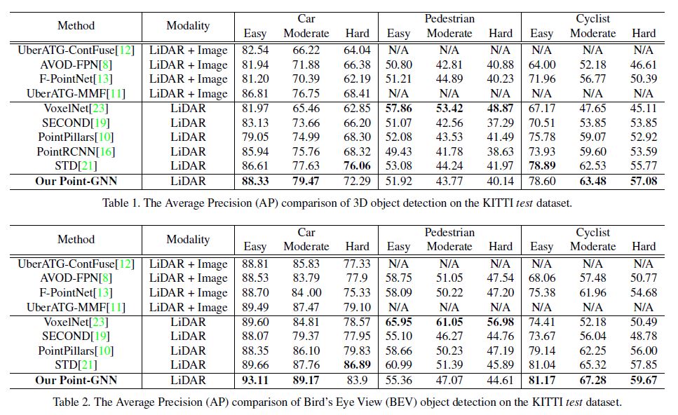
We have submitted our results to the KITTI 3D object detection benchmark and the Bird’s Eye View (BEV) object detection benchmark.
In Table 1 and Table 2, we compare our results with the existing literature.
The KITTI dataset evaluates the Average Precision (AP) on three difficulty levels: Easy, Moderate, and Hard.
Our approach achieves the leading results on the Car detection of Easy and Moderate level and also the Cyclist detection of Moderate and Hard level.
Remarkably, on the Easy level BEV Car detection, we surpass the previous state-of-the-art approach by 3.45.
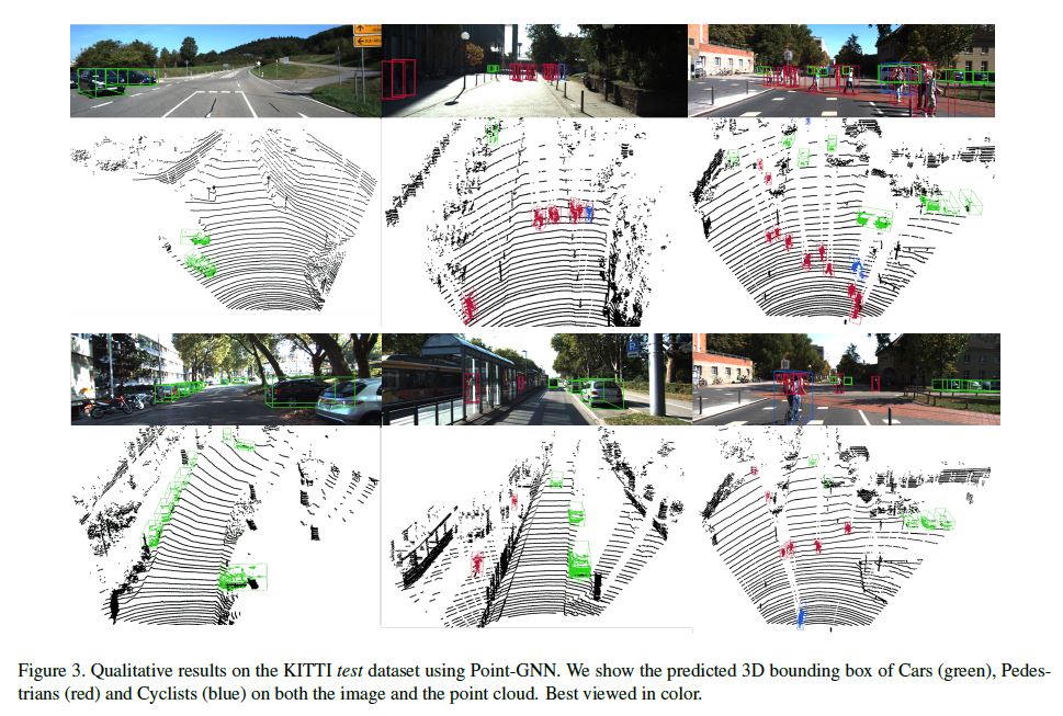
Also, we outperform fusion-based algorithms in all categories except for Pedestrian detection. In Figure 3, we provide qualitative detection results on all categories.
The results on both the camera image and the point cloud can be visualized.
It must be noted that our approach uses only the point cloud data.
The camera images are purely used for visual inspection since the test dataset does not provide ground truth labels.
As shown in Figure 3, our approach still detects Pedestrian reasonably well despite not achieving the top score.
One likely reason why Pedestrian detection is not as good as that for Car and Cyclist is that the vertices are not dense enough to achieve more accurate bounding boxes.

우리는 결과를 KITTI 3D object detection benchmark와 BEV(Bird’s Eye View) object detection benchmark에 제출했다.
Table 1과 Table 2에서는 우리의 결과를 기존 문헌과 비교한다.
KITTI dataset는 세 가지 난이도로 Average Precision (AP)를 평가한다: Easy, Moderate, Hard.
우리의 접근 방식은 Easy level과 Moderate level의 Car detection와 Moderate 및 Hard level의 Cyclist detection에서 선도적인 결과를 달성한다.
놀랍게도, Easy level BEV Car detection에서, 우리는 이전의 state-of-the-art 접근 방식을 3.45만큼 능가한다.
또한 Pedestrian detection를 제외한 모든 범주에서 fusion-based algorithms을 능가한다.
그림 3에서는 모든 범주에 대한 qualitative detection 결과를 제공한다.
camera image와 point cloud에 대한 결과를 시각화할 수 있다.
우리의 접근 방식은 point cloud data만 사용한다는 점에 유의해야 한다.
test dataset가 ground truth labels을 제공하지 않기 때문에 camera images는 시각적 검사에 순수하게 사용된다.
Figure 3에서와 같이, 우리의 접근 방식은 최고 점수를 달성하지 못했지만 여전히 보행자를 합리적으로 잘 감지한다.
보행자 감지가 자동차와 사이클리스트의 그것만큼 좋지 않은 한 가지 가능한 이유는 vertices가 더 정확한 bounding boxes를 달성할 수 있을 만큼 조밀(dense)하지 않기 때문이다.

4.4. Ablation Study

For the ablation study, we follow the standard practice [10][21][5] and split the training samples into a training split of 3712 samples and a validation split of 3769 samples.
We use the training split to train the network and evaluate its accuracy on the validation split.
We follow the same protocol and assess the accuracy by AP.
Unless explicitly modified for a controlled experiment, the network configuration and training parameters are the same as those in the previous section.
We focus on the detection of Car because of its dominant presence in the dataset.

ablation study의 경우 표준 관행[10][21][5]을 따르고 training 샘플을 3712 샘플의 training split와 3769 샘플의 validation split으로 분할한다.
우리는 network를 훈련시키고 validation split에 대한 정확성을 평가하기 위해 training split을 사용한다.
우리는 동일한 protocol을 따르고 AP로 정확도를 평가한다.
통제된 실험에 대해 명시적으로 수정되지 않는 한, network configuration 및 training parameters는 이전 절과 동일하다.
우리는 dataset에서 차의 지배적인 존재 때문에 자동차의 탐지에 초점을 맞춘다.

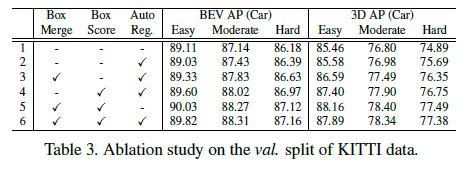
Box merging and scoring. In Table 3, we compare the object detection accuracy with and without box merging and scoring.
For the test without box merging, we modify line 11 in Algorithm 1.
Instead of taking the median bounding box, we directly take the bounding box with the highest classification score as in standard NMS.
For the test without box scoring, we modify lines 12 and 13 in Algorithm 1 to set the highest classification score as the box score.
For the test without box merging or scoring, we modify lines 11, 12, and 13, which essentially leads to standard NMS.
Row 2 of Table 3 shows a baseline implementation that uses standard NMS with the auto-registration mechanism.
As shown in Row 3 and Row 4 of Table 3, both box merging and box scoring outperform the baseline.
When combined, as shown in Row 6 of the table, they further outperform the individual accuracy in every category.
Similarly, when not using auto-registration, box merging and box scoring (Row 5) also achieve higher accuracy than standard NMS (Row 1).
These results demonstrate the effectiveness of the box scoring and merging.

Table 3에서는 box merging 및 scoring을 사용한 경우와 사용하지 않은 경우의 object detection 정확도를 비교한다.
box merging이 없는 test의 경우, Algorithm 1에서 line 11을 수정한다.
median bounding box를 사용하는 대신, 표준 NMS에서와 같이 classification score가 가장 높은 bounding box를 직접 취한다.
box scoring 없는 test에서, Algorithm 1에서 12, 13번 라인을 수정하여 가장 높은 classification score를 box score로 설정한다.
box merging 또는 scoring이 없는 test의 경우, 11, 12, 13 라인을 수정하여 기본적으로 standard NMS로 이끈다.
Table 3의 2행에는 auto-registration mechanism과 함께 standard NMS를 사용하는 baseline 구현을 보여준다.
Table 3의 3행과 4행에서 볼 수 있듯이, box merging과 box scoring 모두 baseline보다 성능이 우수하다.
Table 3의 6행과 같이 조합하면, 모든 범주의 개별 정확도를 더욱 능가한다.
마찬가지로, auto-registration을 사용하지 않을 경우 box merging 및 box scoring (Row 5)도 standard NMS (Row 1)보다 높은 정확도를 달성한다.
이러한 결과는 box scoring 및 merging의 효과를 보여준다.

Auto-registration mechanism.
Table 3 also shows the accuracy improvement from the auto-registration mechanism.
As shown in Row 2, by using auto-registration alone, we also surpass the baseline without auto-registration (Row 1) on every category of 3D detection and the moderate and hard categories of BEV detection.
The performance on the easy category of BEV detection decreases slightly but remains close. Combining the auto-registration mechanism with box merging and scoring (Row 6), we achieve higher accuracy than using the auto-registration alone (Row 2).
However, the combination of all three modules (Row 6) does not outperform box merging and score (Row 5).
We hypothesize that the regularization likely needs to be tuned after adding the auto-registration branch.

Table 3은 auto-registration mechanism의 정확도 향상도 보여줍니다.
Row 2에서 볼 수 있듯이, auto-registration만 사용하여 3D detection의 모든 범주와 BEV detection의 moderate 및 hard 범주에서 auto-registration (Row 1)이 없는 baseline도 능가한다.
BEV detection의 easy 범주에서의 성능은 약간 감소하지만 근접한 상태를 유지한다.
auto-registration mechanism을 box merging 과 scoring (Row 6)과 결합하면, auto-registration만 사용하는 것보다 높은 정확도를 달성한다(Row 2).
그러나 세 modules의 조합(Row 6)이 box merging 및 score (Row 5)를 능가하지는 않는다.
우리는 auto-registration branch를 추가한 후 정규화를 조정할 필요가 있을 것으로 가정한다.

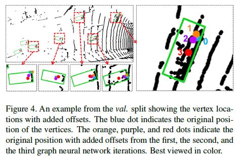
We further investigate the auto-registration mechanism by visualizing the offset \(\Delta x\) in Equation 4.
We extract \(\Delta x\) from different GNN iterations and add them to the vertex position. Figure 4 shows the vertices that output detection results and their positions with added offsets.
We observe that the vertex positions with added offsets move towards the center of vehicles. We see such behaviors regardless of the original vertex position.
In other words, when the GNN gets deeper, the relative coordinates of the neighbor vertices depend less on the center vertex position but more on the property of the point cloud.
The offset \(\Delta x\) cancels the translation of the center vertex, and thus reduces the sensitivity to the vertex translation.
These qualitative results demonstrate that Equation 4 helps to reduce the translation variance of vertex positions

우리는 Equation 4에서 offset \(\Delta x\)를 시각화하여 auto-registration mechanism을 추가로 조사한다.
우리는 서로 다른 GNN iterations에서 \(\Delta x\)를 추출하고 vertex position에 그것들을 추가한다.
Figure 4는 detection 결과를 출력하는 vertices와 offsets이 추가된 vertices와의 positions를 보여준다.
우리는 offsets이 추가된 vertex positions가 vehicles 중심을 향해 이동한다는 것을 관찰한다.
우리는 original vertex position에 관계없이 그러한 행동을 본다.
다시 말해서, GNN이 더 깊어지면, 인접 vertex의 상대 좌표는 중심 vertex 위치에 덜 의존하지만 point cloud의 property(속성)에 더 많이 의존한다.
offset \(\Delta x\)는 중심 vertex의 translation을 취소하므로 vertex 변환에 대한 민감도를 감소시킨다.
이러한 qualitative results는 Equation 4가 vertex 위치의 translation variance을 줄이는 데 도움이 된다는 것을 보여준다.

Point-GNN iterations.
Our Point-GNN refine the vertex states iteratively.
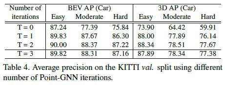
In Table 4, we study the impact of the number of iterations on the detection accuracy.
We train Point-GNNs with T = 1, T = 2, and compare them with T = 3, which is the configuration in Section 4.3.1.
Additionally, we train a detector using the initial vertex state directly without any Point-GNN iteration.
As shown in Table 4, the initial vertex state alone achieves the lowest accuracy since it only has a small receptive field around the vertex.
Without Point-GNN iterations, the local information cannot flow along the graph edges, and therefore its receptive field cannot expand.
Even with a single Point-GNN iteration T = 1, the accuracy improves significantly.
T = 2 has higher accuracy than T = 3, which is likely due to the training difficulty when the neural network goes deeper.

우리의 Point-GNN은 vertex states를 반복적으로 다듬는다.
Table 4에서는 반복 횟수가 detection 정확도에 미치는 영향을 연구한다.
우리는 T = 1, T = 2를 사용하여 Point-GNN을 train하고 이를 T = 3과 비교한다.
또한, 우리는 Point-GNN iteration 없이 initial vertex state를 직접 사용하여 detector를 train시킨다.
Table 4에서 보듯이, initial vertex state만으로도 vertex 주위에 small receptive field만 있기 때문에 가장 낮은 정확도를 달성한다.
Point-GNN iteration이 없으면, local information가 graph edges를 따라 flow할 수 없으므로 수신 필드를 확장할 수 없다.
단일 Point-GNN 반복 T = 1을 사용하더라도 정확도는 크게 향상된다.
T = 2는 T = 3보다 정확도가 높으며, 이는 신경망이 더 깊어질 때 훈련 난이도로 인해 발생할 수 있다.

Running-time analysis. The speed of the detection algorithm is important for real-time applications such as autonomous driving.
However, multiple factors affect the running time, including algorithm architecture, code optimization and hardware resource.
Furthermore, optimizing the implementation is not the focus of this work.
However, a breakdown of the current inference time helps with future optimization.
Our implementation is written in Python and uses Tensorflow for GPU computation.
We measure the inference time on a desktop with Xeon E5-1630 CPU and GTX 1070 GPU.
The average processing time for one sample in the validation split is 643ms.
Reading the dataset and running the calibration takes 11.0% time (70ms).
Creating the graph representation consumes 18.9% time (121ms). The inference of the GNN takes 56.4% time (363ms).
Box merging and scoring take 13.1% time (84ms).

Robustness on LiDAR sparsity The KITTI dataset collects point cloud data using a 64-scanning-line LiDAR.
Such a high-density LiDAR usually leads to a high cost.
Therefore, it is of interest to investigate the object detection performance in a less dense point cloud.
To mimic a LiDAR system with fewer scanning lines, we downsample the scanning lines in the KITTI validation dataset.
Because KITTI gives the point cloud without the scanning line information, we use k-means to cluster the elevation angles of points into 64 clusters, where each cluster represents a LiDAR scanning line.
We then downsample the point cloud to 32, 16, 8 scanning lines by skipping scanning lines in between.
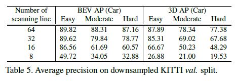
Our test results on the downsampled KITTI validation split are shown in Table 5.
The accuracy for the moderate and hard levels drops fast with downsampled data, while the detection for the easy level data maintains a reasonable accuracy until it is downsampled to 8 scanning lines.
This is because that the easy level objects are mostly close to the LiDAR, and thus have a dense point cloud even if the number of scanning lines drops.

KITTI 데이터 세트는 64-scanning-line LiDARR을 사용하여 point cloud data를 수집한다.
이러한 고밀도 LiDAR은 일반적으로 높은 비용으로 이어진다.
따라서 저밀도 point cloud에서 object detection 성능을 조사하는 것이 중요하다.
더 적은 수의 scanning lines을 가진 LiDAR 시스템을 모방하기 위해, KITTI validation dataset에서 scanning lines을 downsample한다.
KITTI는 scanning line 정보 없이 point cloud을 제공하기 때문에 k-means을 사용하여 points의 elevation angles를 64개 군집으로 클러스터링하며, 여기서 각 군집은 LiDAR scanning line을 나타낸다.
그런 다음 중간에서 scanning lines을 skipping하여 point cloud를 32, 16, 8개의 scanning lines으로 downsample한다.
downsample된 KITTI validation split에 대한 우리의 테스트 결과는 Table 5에 나와 있다.
moderate 및 hard levels에 대한 정확도는 다운샘플링된 data를 사용하여 빠르게 떨어지는 반면, easy level data에 대한 detection은 8개의 scanning lines로 다운샘플링될 때까지 적절한 정확도를 유지한다.
이는 easy level objects가 대부분 LiDAR에 가깝기 때문에 scanning lines 수가 떨어져도 point cloud가 조밀하기 때문이다.

5. Conclusion

We have presented a graph neural network, named Point-GNN, to detect 3D objects from a graph representation of the point cloud.
By using a graph representation, we encode the point cloud compactly without mapping to a grid or sampling and grouping repeatedly.
Our Point-GNN achieves the leading accuracy in both the 3D and Bird’s Eye View object detection of the KITTI benchmark.
Our experiments show the proposed auto-registration mechanism reduces transition variance, and the box merging and scoring operation improves the detection accuracy.
In the future, we plan to optimize the inference speed and also fuse the inputs from other sensors.

point cloud의 graph representation에서 3D objects를 detect하기 위해 Point-GNN이라는 graph neural network을 제시하였다.
graph representation을 사용하여 grid에 mapping하거나 sampling 및 grouping를 반복하지 않고 point cloud를 압축적으로 인코딩한다.
우리의 Point-GNN은 KITI benchmark의 3D 및 Bird’s Eye View object detection 모두에서 최고의 정확도를 달성한다.
우리의 실험은 제안된 auto-registration mechanism이 transition variance을 줄이고 box merging 및 scoring operation을 통해 감지 정확도를 향상시킨다는 것을 보여준다.
미래에는 추론 속도를 최적화하고 다른 센서의 입력을 융합할 계획이다.