ICCV 2019 paper

• Abstract
• 1. Introduction
• 2. Related Work
• 3. Cross View Fusion for 2D Pose Estimation
  • 3.1. Implementation
  • 3.2. Limitation and Solution
• 4. RPSM for Multi-view 3D Pose Estimation
  • 4.1. Pictorial Structure Model
  • 4.2. Recursive Pictorial Structure Model
  • 4.3. Relation to Bundle Adjustment [25]
• 5. Datasets and Metrics
• 6. Experiments on 2D Pose Estimation
  • 6.1. Implementation Details
  • 6.2. Quantitative Results
  • 6.3. Qualitative Results
• 7. Experiments on 3D Pose Estimation
  • 7.1. Implementation Details
  • 7.2. Quantitative Results
  • 7.3. Qualitative Results
  • 7.4. Generalization to the Total Capture Dataset
  • 7.5. Generalization to New Camera Setups
• 8. Conclusion

Abstract

We present an approach to recover absolute 3D human poses from multi-view images by incorporating multi-view geometric priors in our model. It consists of two separate steps: (1) estimating the 2D poses in multi-view images and (2) recovering the 3D poses from the multi-view 2D poses.

우리는 모델에 multi-view geometric 사전확률을 통합하여 multi-view images에서 absolute 3D human poses를 recover하는 접근 방식을 제시한다.
이 단계는 두 단계로 구성됩니다. (1) multi-view images에서 2D poses를 estimating하는 것과 (2) multi-view 2D poses에서 3D poses를 recovering하는 것입니다.

First, we introduce a cross-view fusion scheme into CNN to jointly estimate 2D poses for multiple views.
Consequently, the 2D pose estimation for each view already benefits from other views.
Second, we present a recursive Pictorial Structure Model to recover the 3D pose from the multi-view 2D poses.
It gradually improves the accuracy of 3D pose with affordable computational cost.
We test our method on two public datasets H36M and Total Capture.
The Mean Per Joint Position Errors on the two datasets are 26mm and 29mm, which outperforms the state-of-the-arts remarkably (26mm vs 52mm, 29mm vs 35mm).

첫째, 우리는 multiple views를 위해 2D poses를 jointly로 estimate하기 위해 CNN에 cross-view fusion scheme를 도입한다.
결과적으로 각 view에 대한 2D pose estimation은 이미 다른 뷰에서 이익을 얻는다.
둘째, multi-view 2D poses에서 3D pose를 recover하기 위한 recursive Pictorial Structure Model을 제시한다.
저렴한 계산 비용으로 3D 포즈의 정확도를 단계적으로 향상시킨다.
우리는 두 개의 공개 데이터 세트 H36M과 Total Capture에서 우리의 방법을 테스트한다.
두 데이터 세트의 Mean Per Joint Position Errors는 26mm와 29mm로 state-of-the-arts 상태(26mm vs 52mm, 29mm vs 35mm)를 크게 능가한다.

1. Introduction

The task of 3D pose estimation has made significant progress due to the introduction of deep neural networks.
Most efforts [16, 13, 33, 17, 23, 19, 29, 28, 6] have been devoted to estimating relative 3D poses from monocular images.
The estimated poses are centered around the pelvis joint thus do not know their absolute locations in the environment (world coordinate system).

3D pose estimation 작업은 deep neural networks의 도입으로 인해 상당한 진전을 이루었다.
대부분의 노력[16, 13, 33, 17, 23, 19, 29, 28, 6]은 단안 영상에서 상대적인 3D poses를 추정하는 데 사용되었다.
추정된 포즈는 골반 관절의 중심에 있으므로 환경(world coordinate system)에서 절대적인 위치를 알 수 없다.

In this paper, we tackle the problem of estimating absolute 3D poses in the world coordinate system from multiple cameras [1, 15, 4, 18, 3, 20].
Most works follow the pipeline of first estimating 2D poses and then recovering 3D pose from them.
However, the latter step usually depends on the performance of the first step which unfortunately often has large errors in practice especially when occlusion or motion blur occurs in images.
This poses a big challenge for the final 3D estimation.

본 논문에서는 여러 카메라[1, 15, 4, 18, 3, 20]를 사용한 world coordinate system에서 absolute 3D poses를 추정하는 문제를 다룬다.
대부분의 작업은 먼저 2D 포즈를 추정한 다음 3D 포즈를 복구하는 파이프라인을 따른다.
그러나 후자는 일반적으로 첫 번째 단계의 성능에 따라 달라지는데, 안타깝게도 첫 번째 단계의 성능은 특히 영상에 occlusion 또는 motion blur 현상이 발생할 때 실제로 큰 오류를 범하는 경우가 많다.
이는 최종 3D estimation에 큰 문제를 제기한다.

On the other hand, using the Pictorial Structure Model (PSM) [14, 18, 3] for 3D pose estimation can alleviate the influence of inaccurate 2D joints by considering their spatial dependence.
It discretizes the space around the root joint by an N ×N ×N grid and assigns each joint to one of the \(N^3\) bins (hypotheses).
It jointly minimizes the projection error between the estimated 3D pose and the 2D pose, along with the discrepancy of the spatial configuration of joints and its prior structures.
However, the space discretization causes large quantization errors.
For example, when the space surrounding the human is of size 2000mm and N is 32, the quantization error is as large as 30mm. We could reduce the error by increasing N, but the inference cost also increases at \(O(N^3)\), which is usually intractable.

반면, 3D pose estimation을 위해 Pictorial Structure Model (PSM)[14, 18, 3]을 사용하면 공간 의존성을 고려하여 부정확한 2D joints의 영향을 완화할 수 있다.
N × N × N grid에 의해 뿌리 관절 주변의 공간을 이산화하고 각 관절을 \(N^3\) bins 중 하나에 할당한다.(hypotheses)
관절의 공간 구성과 이전 구조의 불일치와 함께, estimated 3D pose와 2D pose 사이의 projection error를 jointly로 최소화한다.
그러나 공간 이산화는 큰 양자화 오류를 일으킨다.
예를 들어 인간을 둘러싼 공간이 2000mm이고 N이 32인 경우 정량화 오류는 30mm만큼 크다.
우리는 N을 증가시켜 오차를 줄일 수 있지만, 추론 비용 또한 대개 다루기 힘든 O(\(N^3\))에서 증가한다.

Second, we present Recursive Pictorial Structure Model (RPSM), to recover the 3D pose from the estimated multi-view 2D pose heatmaps.
Different from PSM which directly discretizes the space into a large number of bins in order to control the quantization error, RPSM recursively discretizes the space around each joint location (estimated in the previous iteration) into a finer-grained grid using a small number of bins.
As a result, the estimated 3D pose is refined step by step.
Since N in each step is usually small, the inference speed is very fast for a single iteration.
In our experiments, RPSM decreases the error by at least 50% compared to PSM with little increase of inference time.

둘째, estimated multi-view 2D pose heatmaps에서 3D pose를 recover하기 위해 Recursive Pictorial Structure Model (RPSM)을 제시합니다.
quantization error를 제어하기 위해 공간을 직접 많은 수의 bins으로 이산시키는 PSM과는 달리, RPSM은 적은 수의 bins을 사용하여 각 관절 위치(estimated in the previous iteration) 주변의 공간을 finer-grained grid로 재귀적 이산화한다.

For 2D pose estimation on the H36M dataset [11], the average detection rate over all joints improves from 89% to 96%.
The improvement is significant for the most challenging “wrist” joint.
For 3D pose estimation, changing PSM to RPSM dramatically reduces the average error from 77mm to 26mm.
Even compared with the state-of-the-art method with an average error 52mm, our approach also cuts the error in half.
We further evaluate our approach on the Total Capture dataset [27] to validate its generalization ability.
It still outperforms the state-of-the-art [26].

H36M 데이터 세트에 대한 2D 포즈 추정의 경우 [11], 모든 관절에 대한 평균 감지 속도는 89%에서 96%로 향상된다.
개선은 가장 도전적인 “손목” 관절에 중요하다.
3D 포즈 추정의 경우 PSM을 RPSM으로 변경하면 평균 오차가 77mm에서 26mm로 크게 줄어든다.
평균 오차 52mm의 최첨단 방법과 비교해도 우리의 접근 방식은 오류를 절반으로 줄인다.
우리는 총 캡처 데이터 세트[27]에 대한 접근 방식을 추가로 평가하여 일반화 능력을 검증한다.
그것은 여전히 최첨단[26]을 능가한다.

2. Related Work

We first review the related work on multi-view 3D pose estimation and discuss how they differ from our work.
Then we discuss some techniques on feature fusion.

먼저 multi-view 3D pose estimation에 대한 관련 작업을 검토하고 작업과 어떻게 다른지 논의한다.
그런 다음 feature fusion에 대한 몇 가지 기술에 대해 논의한다.

Multi-view 3D Pose Estimation
Many approaches [15, 10, 4, 18, 3, 19, 20] are proposed for multi-view pose estimation.
They first define a body model represented as simple primitives, and then optimize the model parameters to align the projections of the body model with the image features.
These approaches differ in terms of the used image features and optimization algorithms.

multi-view pose estimation을 위해 많은 접근 방식[15, 10, 4, 18, 3, 19, 20]이 제안된다.
이들은 먼저 simple primitives로 표현되는 body model을 정의한 다음, body model의 projections을 image features과 정렬하도록 model parameters를 최적화한다.
이러한 접근 방식은 사용된 image features과 최적화 알고리즘 측면에서 다르다.

We focus on the Pictorial Structure Model (PSM) which is widely used in object detection [8, 9] to model the spatial dependence between the object parts.
This technique is also used for 2D [32, 5, 1] and 3D [4, 18] pose estimation where the parts are the body joints or limbs.
In [1], Amin et al. first estimate the 2D poses in a multi-view setup with PSM and then obtain the 3D poses by direct triangulation.
Later Burenius et al. [4] and Pavlakos et al. [18] extend PSM to multi-view 3D human pose estimation.
For example, in [18], they first estimate 2D poses independently for each view and then recover the 3D pose using PSM.
Our work differs from [18] in that we extend PSM to a recursive version, i.e. RPSM, which efficiently refines the 3D pose estimations step by step.
In addition, they [18] do not perform cross-view feature fusion as we do.

우리는 object detection [8, 9]에서 object parts 사이의 공간 의존성을 모델링하기 위해 널리 사용되는 Pictorial Structure Model (PSM)에 초점을 맞춘다.
이 기술은 또한 신체 관절이나 팔다리가 있는 부분이 2D [32, 5, 1] 및 3D [4, 18] pose estimation에도 사용된다.
[1]에서 Amin 등은 PSM이 있는 multi-view 설정에서 먼저 2D poses를 추정한 다음 직접 삼각측정을 통해 3D poses를 얻는다.
나중에 Burenius 외 [4]와 Pavlakos 외 [18]는 PSM을 multi-view 3D human pose estimation으로 확장한다.
예를 들어, [18]에서는 먼저 각 view에 대해 독립적으로 2D poses를 추정한 다음 PSM을 사용하여 3D pose를 recover한다.
우리의 연구는 PSM을 recursive version, 즉 RPSM으로 확장한다는 점에서 [18]과 다르다. RPSM은3D pose estimations을 단계별로 효율적으로 세분화한다.
또한 [18]은(는) cross-view feature fusion을 수행하지 않는다.

Multi-image Feature Fusion
Fusing features from different sources is a common practice in the computer vision literature.
For example, in [34], Zhu et al. propose to warp the features of the neighboring frames (in a video sequence) to the current frame according to optical flow in order to robustly detect the objects.
Ding et al. [7] propose to aggregate the multi-scale features which achieves better segmentation accuracy for both large and small objects.

다른 sources의 features들을 융합하는 것은 computer vision literature에서 흔한 관행이다.
예를 들어, [34]에서 Zhu 등은 objects를 robustly하게 detect하기 위해 optical flow에 따라 인접 프레임의 features(비디오 시퀀스로)을 현재 프레임으로 왜곡할 것을 제안한다.
Ding 등. [7]은 큰 객체와 작은 객체 모두에 대해 더 나은 segmentation accuracy를 달성하는 multi-scale features을 집계할 것을 제안한다.

Amin et al. [1] propose to estimate 2D poses by exploring the geometric relation between multi-view images.
It differs from our work in that it does not fuse features from other views to obtain better 2D heatmaps.
Instead, they use the multi-view 3D geometric relation to select the joint locations from the “imperfect” heatmaps.
In [12], multi-view consistency is used as a source of supervision to train the pose estimation network.
To the best of our knowledge, there is no previous work which fuses multi-view features so as to obtain better 2D pose heatmaps because it is a challenging task to find the corresponding features across different views which is one of our key contributions of this work.

Amin 외. [1]은 multi-view images 간의 geometric 관계를 탐색하여 2D poses를 추정하는 것을 제안한다.
더 나은 2D heatmaps을 얻기 위해 다른 views와 features을 융합하지 않는다는 점에서 우리의 작업과 다르다.
대신 multi-view 3D geometric 관계를 사용하여 “불완전한” heatmaps에서 joint 위치를 선택한다.
[12]에서 multi-view consistency은 pose estimation network를 훈련시키기 위한 supervision의 source로 사용된다.
우리가 아는 한, 이 작업의 key contributions 중 하나인 다른 views에서 해당 features을 찾는 것은 어려운 작업이기 때문에 더 나은 2D pose heatmaps을 얻기 위해 multi-view features을 융합한 previous work는 없다.

3. Cross View Fusion for 2D Pose Estimation

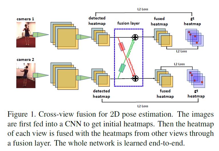
Our 2D pose estimator takes multi-view images as input, generates initial pose heatmaps respectively for each, and then fuses the heatmaps across different views such that the heatmap of each view benefits from others.
The process is accomplished in a single CNN and can be trained end-to-end.
Figure 1 shows the pipeline for two-view fusion.
Extending it to multi-views is trivial where the heatmap of each view is fused with the heatmaps of all other views.
The core of our fusion approach is to find the corresponding features between a pair of views.

우리의 2D pose estimator는 multi-view images을 입력으로 가져가고 각각에 대해 초기 pose heatmaps을 생성한 다음 각 view의 heatmap이 다른 views로부터 benefits을 얻도록 여러 views에 걸쳐 heatmaps을 융합한다.
이 프로세스는 단일 CNN에서 수행되며 end-to-end 훈련을 받을 수 있다.
Figure 1은 two-view fusion을 위한 pipeline이다.
각 view의 heatmap가 다른 모든 views의 heatmaps와 융합되는 경우 multi-views로 확장하는 것은 trivial이다. 우리의 fusion 접근법의 핵심은 한 쌍의 views 사이에서 상응하는 features을 찾는 것이다.

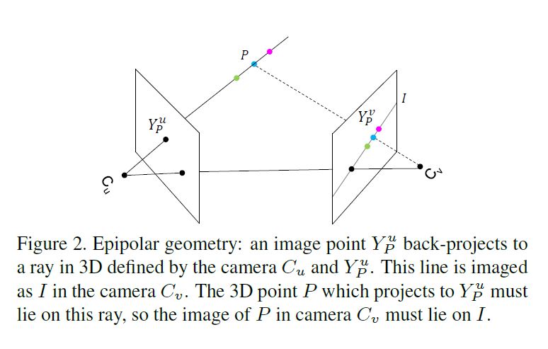
Suppose there is a point \(P\) in 3D space.
See Figure 2.
Its projections in view \(u\) and \(v\) are \(Y_P^u \in \mathcal{Z}^u\) and \(Y^v_P \in Z^v\), respectively where \(\mathcal{Z}^u\) and \(\mathcal{Z}^v\) denote all pixel locations in the two views, respectively.
The heatmaps of view \(u\) and \(v\) are \(\mathcal{F}^u = {x^u_1, ..., x^u_{\vert \mathcal{Z}^u \vert}}\) and \(\mathcal{F}^v = {x^v_1, ..., x^v_{\vert \mathcal{Z}^v \vert}}\).

3D space에 point P가 있다고 가정하자 \(Z^u\)는 view \(u\)의 모든 pixel locations,
\(Z^v\)는 view \(v\)의 모든 pixel locations
\(Y^u_P\)와 \(Y^v_P\)는 Point \(P\)를 각각 \(\mathcal{Z}^u\)와 \(\mathcal{Z}^v\)에 projection 한것 view \(u\)의 heatmap : \(\mathcal{F}^u = {x^u_1, ..., x^u_{\vert \mathcal{Z}^u \vert}}\), view \(v\)의 heatmap : \({F}^v = {x^v_1, ..., x^v_{\vert \mathcal{Z}^v \vert}}\)

(P는 view \(u\)에 \(Y^u_P\)로 투영되고 view \(u\)의 카메라는 \(C_u\)이고 카메라 \(C_u\)와 \(C_v\)를 잇는 선과 영상 평면 view \(u\)와 \(v\)가 만나는 점을 epipole라고 부르고 epipole점과 투영점 (\(Y^u_P, Y^v_P\))을 잇는 직선을 epipolar line이라고 부른다.)

The core idea of fusing a feature in view \(u\), say \(x^u_i\) , with the features from \(\mathcal{F}^v\) is to establish the correspondence between the two views:

view \(u\)의 feature,즉 \(x^u_i\)를 \(\mathcal{F}^v\)의 features과 융합하는 핵심 아이디어는 다음 두 views 사이의 correspondence를 설정하는 것이다.

\[x^u_i \leftarrow x^u_i + \sum^{\vert \mathcal{Z^v} \vert }_{j=1}\omega_{j,i} \cdot x^v_j , \; \forall i \in \mathcal{Z^u}, \; \; \; (1)\]

where \(\omega_{j,i}\) is a to be determined scalar.
Ideally, for a specific \(i\), only one \(\omega_{j,i}\) should be positive, while the rest are zero.
Specifically, \(\omega_{j,i}\) is positive when the pixel \(i\) in view \(u\) and
pixel \(j\) in view \(v\) correspond to the same 3D point.

여기서 \(\omega_{j,i}\)는 결정 스칼라이다.
이상적으로, 특정 \(i\)의 경우, \(\omega_{j,i}\) 하나만 양수여야 하고 나머지는 0이어야 한다.
구체적으로, \(\omega_{j,i}\)는 view \(u\)의 pixel \(i\)가 양수이며
view \(v\)의 pixel \(j\)는 동일한 3D 포인트에 해당한다.

Suppose we know only \(Y^u_P\) , how can we find the corresponding point \(Y^v_P\) in the image of a different view?
We know \(Y^v_P\) is guaranteed to lie on the epipolar line I.
But since we do not know the depth of P, which means it may move on the line defined by \(C_u\) and \(Y^u_P\) , we cannot determine the exact location of \(Y^v_P\) on \(I\).
This ambiguity poses a challenge for the cross view fusion.

\(Y^u_P\)만 알고 있다고 가정하면, 어떻게 다른 view의 이미지에서 해당 점 \(Y^v_P\)을 찾을 수 있는가?
우리는 \(Y^v_P\)가 epipolar line I에 있다는 것을 안다.
그러나 우리는 \(P\)의 깊이를 모르기 때문에 \(P\)가 \(C_u\)와 \(Y^u_P\)에 의해 정의된 라인에서 이동할 수 있으므로 \(I\)에서 \(Y^v_P\)의 정확한 위치를 결정할 수 없다.
이러한 모호성은 cross view fusion에 문제를 제기한다.

Our solution is to fuse xu i with all features on the line I. This may sound brutal at the first glance, but is in fact elegant. Since fusion happens in the heatmap layer, ideally, xv j should have large response at Y v P (the cyan point) and zeros at other locations on the epipolar line I. It means the non-corresponding locations on the line will contribute no or little to the fusion. So fusing all pixels on the epipolar line is a simple yet effective solution.

3.1. Implementation

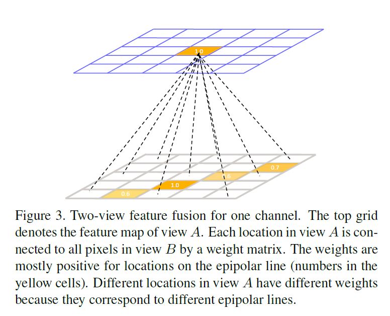
\(x^u_i \leftarrow x^u_i + \sum^{\vert \mathcal{Z^v} \vert }_{j=1}\omega_{j,i} \cdot x^v_j , \; \forall i \in \mathcal{Z^u}, \; \; \; (1)\)
The feature fusion rule (Eq. (1)) can be interpreted as a fully connected layer imposed on each channel of the pose heatmaps where \(\omega\) are the learnable parameters.
Figure 3 illustrates this idea.
Different channels of the feature maps, which correspond to different joints, share the same weights because the cross view relations do not depend on the joint types but only depend on the pixel locations in the camera views.
Treating feature fusion as a neural network layer enables the end-to-end learning of the weights.

feature fusion rule (Eq. (1))은 \(\omega\)가 학습 가능한 parameters인 pose heatmaps의 각 channel에 부과된 fully connected layer으로 해석할 수 있다.
Figure 3은 이러한 생각을 보여준다.
cross view 관계는 joint 유형에 따라 달라지지 않고 카메라 views의 pixel locations에만 의존하기 때문에 다른 joints에 상응하는 feature maps의 다른 channels은 동일한 weights를 공유한다.
feature fusion을 neural network layer로 처리하면 weights의 end-to-end learning을 가능하게 한다.

We investigate two methods to train the network.
In the first approach, we clip the positive weights to zero during training if the corresponding locations are off the epipolar line.
Negative weights are allowed to represent suppression relations.
In the second approach, we allow the network to freely learn the weights from the training data.
The final 2D pose estimation results are also similar for the two approaches.
So we use the second approach for training because it is simpler.

우리는 network를 훈련시키는 두 가지 방법을 조사한다.
첫 번째 접근법에서, 우리는 해당 locations가 epipolar line으로부터 벗어날 경우 훈련 중에 positive weights를 0으로 clip한다.
Negative weights는 억제 관계를 나타낼 수 있다.
두 번째 접근법에서는 network가 훈련 데이터에서 weights를 자유롭게 학습할 수 있도록 한다.
최종 2D pose estimation 결과도 두 접근법에 대해 유사하다.
그래서 우리는 두 번째 접근법이 더 간단하기 때문에 두번째 접근법을 훈련에 사용한다.

3.2. Limitation and Solution

The learned fusion weights which implicitly encode the information of epipolar geometry are dependent on the camera configurations.
As a result, the model trained on a particular camera configuration cannot be directly applied to another different configuration.

epipolar geometry의 정보를 암묵적으로 encode하는 학습된 fusion weights는 카메라 configurations에 따라 달라진다.
따라서, 특정 카메라 구성에 대해 훈련된 모델을 다른 구성에 직접 적용할 수 없다.

We propose an approach to automatically adapt our model to a new environment without any annotations.
We adopt a semi-supervised training approach following the previous work [21].
First, we train a single view 2D pose estimator [31] on the existing datasets such as MPII which have ground truth pose annotations.
Then we apply the trained model to the images captured by multiple cameras in the new environment and harvest a set of poses as pseudo labels.
Since the estimations may be inaccurate for some images, we propose to use multi-view consistency to filter the incorrect labels.
We keep the labels which are consistent across different views following [21].
In training the cross view fusion network, we do not enforce supervision on the filtered joints.
We will evaluate this approach in the experiment section.

우리는 아무런 annotations(라벨,주석,답) 없이 우리의 모델을 새로운 환경에 자동으로 적응시키는 접근법을 제안한다.
우리는 이전 연구[21]에 이어 semi-supervised training approach를 채택한다.
먼저, 우리는 ground truth pose annotations을 가지는 MPII와 같은 기존 데이터 세트에 대해 single view 2D pose estimator[31]를 훈련시킨다.
그런 다음 훈련된 모델을 새로운 환경에서 여러 카메라가 캡처한 이미지에 적용하고 일련의 포즈를 pseudo labels로 수집한다.
일부 이미지의 경우 estimations가 inaccurate할 수 있으므로, multi-view 일관성을 사용하여 incorrect labels을 필터링할 것을 제안한다.
우리는 [21] 이후 서로 다른 views에 걸쳐 일관된 labels을 유지한다.
cross view fusion network를 훈련시킬 때, 우리는 필터링된 joints에 대한 supervision을 시행하지 않는다.
우리는 실험 섹션에서 이 접근 방식을 평가할 것이다.

4. RPSM for Multi-view 3D Pose Estimation

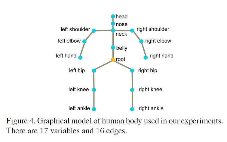
We represent a human body as a graphical model with \(M\) random variables \(\mathcal{J} = \{J_1, J_2, · · · , J_M\}\) in which each variable corresponds to a body joint.
Each variable \(J_i\) defines a state vector \(J_i = [x_i, y_i, z_i]\) as the 3D position of the body joint in the world coordinate system and takes its value from a discrete state space.
See Figure 4. An edge between two variables denotes their conditional dependence and can be interpreted as a physical constraint.

우리는 human body를 graphical model M을 통해 body joint에 대응되는 각 variable인 random variables \(\mathcal{J} = \{J_1, J_2, · · · , J_M\}\)로 나타낸다.

4.1. Pictorial Structure Model

Given a configuration of 3D pose \(\mathcal{J}\) and multi-view 2D pose heatmaps \(\mathcal{F}\), the posterior becomes [3]: \[p(\mathcal{J} \vert \mathcal{F}) = \frac{1}{Z(\mathcal{F})} \prod_{i=1}^M \phi^{\text{conf}}_i(J_i,\mathcal{F}) \prod_{(m,n) \in \varepsilon} \psi^{\text{limb}}(J_m,J_n), \; (2)\]

where \(Z(\mathcal{F})\) is the partition function and \(\varepsilon\) are the graph edges as shown in Figure 4.
The unary potential functions \(\phi^{\text{conf}}_i(J_i,\mathcal{F})\) are computed based on the previously estimated multi-view 2D pose heatmaps \(\mathcal{F}\).
The pairwise potential functions \(\psi^{\text{limb}}(J_m,J_n)\) encode the limb length constraints between the joints.

3D pose의 configuration : \(\mathcal{J}\)
multi-view 2D pose heatmaps : \(\mathcal{F}\)
posterior : (2)
\(Z(\mathcal{F})\) : partition function \(\varepsilon\) : graph edges unary potential functions : \(\phi^{\text{conf}}_i(J_i,\mathcal{F})\) 는 이전에 estimated된 multi-view 2D pose heatmaps \(\mathcal{F}\)
pairwise potential functions \(\psi^{\text{limb}}(J_m,J_n)\)은 joints 간의 팔다리 길이 제약을 인코딩

Discrete state space
We first triangulate the 3D location of the root joint using its 2D locations detected in all views.
Then the state space of the 3D pose is constrained to be within a 3D bounding volume centered at the root joint.
The edge length \(s\) of the volume is set to be 2000mm.
The volume is discretized by an N ×N ×N grid \(\mathcal{G}\).
All body joints share the same state space \(\mathcal{G}\) which consists of \(N^3\) discrete locations (bins).

먼저 모든 views에서 탐지된 2D locations를 사용하여 root joint의 3D location를 삼각 측량한다.
그런 다음 3D pose의 상태 공간은 root joint를 중심으로 한 3D bounding volume 내에 있도록 제한된다.
volume의 edge 길이 \(s\)는 2000mm로 설정된다.
volume은 N × N × N grid \(\mathcal{G}\) 에 의해 discrete화된다.
모든 body joints는 \(N^3\) discrete locations (bins)로 구성된 동일한 상태 공간 \(\mathcal{G}\)를 공유한다.

Unary potentials
Every body joint hypothesis, i.e. a bin in the grid \(\mathcal{G}\), is defined by its 3D position in the world coordinate system.
We project it to the pixel coordinate system of all camera views using the camera parameters, and get the corresponding joint confidence from \(\mathcal{F}\).
We compute the average confidence over all camera views as the unary potential for the hypothesis.

모든 body joint hypothesis, 즉 grid \(\mathcal{G}\)의 bin,은 world coordinate system에서 그것의 3D position에 의해 정의된다.
우리는 카메라 parameters를 사용하여 모든 카메라 views의 pixel 좌표계에 투영하고 \(\mathcal{F}\)에서 해당 joint confidence를 얻는다.
우리는 모든 카메라 views에 대한 평균 confidence를 hypothesis의 unary potential로 계산한다.

Pairwise potentials
Offline, for each pair of joints \((J_m,J_n)\) in the edge set \(\varepsilon\), we compute the average distance \(\tilde{l_{m,n}}\) on the training set as limb length priors.
During inference, the pairwise potential is defined as: \[\psi^{limb}(J_m,J_n) = \begin{cases} 1, \text{if} \; \; l_{m,n} \in [\tilde{l_{m,n}} - \varepsilon, \tilde{l_{m,n}} + \varepsilon] is even \\ 0, \; \; \text{otherwise} \end{cases} \; \; (3)\]

where \(l_{m,n}\) is the distance between \(J_m\) and \(J_n\).
The pairwise term favors 3D poses having reasonable limb lengths.
In our experiments, \(\varepsilon\) is set to be 150mm.

\(l_{m,n}\) : \(J_m\) 와 \(J_n\) 간의 거리
edge set \(\varepsilon\) 에서 each pair of joints : \((J_m,J_n)\) \((J_m,J_n)\)을 위해, 우리는 training sets에서 평균 거리 \(\tilde{l_{m,n}}\)를 팔다리 길이 priors로 계산한다.
Inference 동안, pairwise potential을 다음과 같이 정의된다.
pairwise term는 합리적인 사지 길이를 가진 3D poses를 선호한다. 우리의 실험에서, \(\varepsilon\)는 150mm로 설정되었다.

Inference
The final step is to maximize the posterior (Eq.(2)) over the discrete state space.
Because the graph is acyclic, it can be optimized by dynamic programming with global optimum guarantee.
The computational complexity is of the order of \(\mathcal{O}(N^6)\).

마지막 단계는 discrete 상태 공간에 대한 posterior (Eq.(2))을 최대화하는 것이다.
그래프는 순환적이기 때문에, global optimum 보장을 통해 동적 프로그래밍에 의해 최적화될 수 있다.
계산 복잡성은 \(\mathcal{O}(N^6)\)의 순서이다.

4.2. Recursive Pictorial Structure Model

The PSM model suffers from large quantization errors caused by space discretization.
For example, when we set \(N = 32\) as in the previous work, the quantization error is as large as 30mm (\(i.e. \frac{s}{32×2} \; \text{where} \; \; s = 2000\) is the edge length of the bounding volume).
Increasing \(N\) can reduce the quantization error, but the computation time quickly becomes intractable.
For example, if \(N = 64\), the inference speed will be \(64 = \left( \frac{64}{32} \right)^6\) times slower.

PSM 모델은 공간 이산화로 인해 큰 quantization errors가 발생한다.
예를 들어. 이전 작업에서와 같이 \(N = 32\)로 설정하면 quantization error가 30mm (즉, \(\frac{s}{32×2}\) 여기서 \(s = 2000\)은 bounding volume의 edge length이다).
\(N\)을 늘리면 quantization error를 줄일 수 있지만, 계산 시간은 금방 다루기 어려워진다.
예를 들어, 만약 \(N = 64\)이면, inference speed는 \(64 = \left( \frac{64}{32} \right)^6\)으로 느려진다.

Instead of using a large \(N\) in one iteration, we propose to recursively refine the joint locations through a multiple stage process and use a small \(N\) in each stage.
In the first stage \((t = 0)\), we discretize the 3D bounding volume space around the triangulated root joint using a coarse grid \((N = 16)\) and obtain an initial 3D pose estimation \(L = (L_1, · · · ,L_M)\) using the PSM approach.

하나의 iteration에서 큰 \(N\)을 사용하는 대신, 우리는 다중 단계 과정을 통해 oint locations를 재귀적으로 정제하고 각 단계에서 작은 \(N\)을 사용하는 것을 제안한다.
첫 번째 단계\((t = 0)\)에서는, coarse grid \((N = 16)\)를 이용하여 삼각측량된 root joint 주위의 3D bounding volume space를 이산화하고 PSM approach를 사용한 초기 3D pose estimation \(L = (L_1, · · · ,L_M)\)을 구한다.

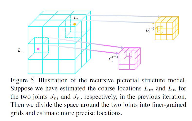
For the following stages \((t ≥ 1)\), for each joint \(J_i\), we discretize the space around its current location \(L_i\) into an 2 × 2 × 2 grid \(G^{(i)}\).
The space discretization here differs from PSM in two-fold.
First, different joints have their own grids but in PSM all joints share the same grid.
See Figure 5 for illustration of the idea.
Second, the edge length of the bounding volume decreases with iterations: \(s_t = \frac{s_t−1}{N}\).
That is the main reason why the grid becomes finer-grained compared to the previous stage.

다음 단계 \((t ≥ 1)\)에 대해, 각 joint \(J_i\)에 대해, current location \(L_i\) 주변의 공간을 2 × 2 × 2 grid \(G^{(i)}\)로 이산화한다.
여기서 공간 이산화는 PSM과 두 가지 면에서 다르다.
첫째, 다른 joints는 그것들 자체 그리드를 가지고 있지만 PSM에서는 모든 joints가 동일한 그리드를 공유한다.
둘째, bounding volume의 edge 길이는 \(s_t = \frac{s_t−1}{N}\) iterations에 따라 감소한다.
그것이 그리드가 이전 단계에 비해 미세해지는 주된 이유이다.

Instead of refining each joint independently, we simultaneously refine all joints considering their spatial relations.
Recall that we know the center locations, sizes and the number of bins of the grids.
So we can calculate the location of every bin in the grids with which we can compute the unary and pairwise potentials.
It is worth noting that the pairwise potentials should be computed on the fly because it depends on the previously estimated locations.
However, because we set N to be a small number (two in our experiments), this computation is fast.

각 joint를 독립적으로 정제하는 대신, 공간 관계를 고려하여 모든 joints를 동시에 정제한다.
그리드의 center locations, sizes와 bins의 수를 알고 있음을 Recall.
그래서 우리는 그리드에 있는 모든 bin의 위치를 계산해서 unary potential과 pairwise potential를 계산할 수 있다.
pairwise potentials는 이전에 estimated locations에 따라 달라지기 때문에 즉시 계산해야 한다는 점에 유의할 필요가 있다.
그러나 \(N\)을 작은 수(실험에서 2개)로 설정하기 때문에 이 계산은 빠르다.

4.3. Relation to Bundle Adjustment [25]

Bundle adjustment [25] is also a popular tool for refining 3D reconstructions.
RPSM differs from it in two aspects.
First, they reach different local optimums due to their unique ways of space exploration.
Bundle adjustment explores in an incremental way while RPSM explores in a divide and conquer way.
Second, computing gradients by finite-difference in bundle adjustment is not stable because most entries of heatmaps are zeros.

Bundle adjustment [25]은 3D reconstructions을 미세화하는 데 널리 사용되는 도구이기도 하다.
RPSM은 두 가지 측면에서 그것과 다르다.
첫째, 그것들은 space 탐험의 독특한 방법으로 인해 다른 지역 최적점에 도달한다.
Bundle adjustment은 점진적으로 탐색하는 반면 RPSM은 분할되고 정복되는 방식으로 탐색한다.
둘째, Bundle adjustment의 finite-difference에 의한 gradients 계산은 heatmaps 대부분의 항목이 0이기 때문에 안정적이지 않다.

5. Datasets and Metrics

The H36M Dataset [11]
We use a cross-subject evaluation scheme where subjects 1, 5, 6, 7, 8 are used for training and 9, 11 for testing.
We train a single fusion model for all subjects because their camera parameters are similar.
In some experiments (which will be clearly stated), we also use the MPII dataset [2] to augment the training data.
Since this dataset only has monocular images, we do not train the fusion layer on these images.

우리는 subjects 1, 5, 6, 7, 8이 training에 사용되고 9, 11이 testing에 사용되는 cross-subject evaluation scheme를 사용한다.
우리는 모든 subjects의 카메라 매개 변수가 유사하기 때문에 모든 subjects에 대해 single fusion model을 훈련시킨다.
일부 실험에서는(분명히 언급될) MPII dataset[2]를 사용하여 training data를 증강한다.
이 데이터 세트에는 단안 영상만 있기 때문에 이러한 영상에 대해 fusion layer을 교육하지 않는다.

The Total Capture Dataset [27]
we also evaluate our approach on the Total Capture dataset to validate its general applicability to other datasets.
Following the previous work [27], the training set consists of “ROM1,2,3”, “Walking1,3”, “Freestyle1,2”, “Acting1,2”, “Running1” on subjects 1,2 and 3.
The testing set consists of “Freestyle3 (FS3)”, “Acting3 (A3)” and “Walking2 (W2)” on subjects 1,2,3,4 and 5.
We use the data of four cameras (1,3,5,7) in experiments.
We do not use the IMU sensors.
We do not use the MPII dataset for training in this experiment.
The hyper-parameters for training the network are kept the same as those on the H36M dataset.

또한 Total Capture dataset에 대한 접근 방식을 평가하여 다른 datasets에 대한 일반적인 적용 가능성을 검증한다.
이전 연구[27]에 이어, training set는 subjects 1, 2, 3에 대해 “ROM1,2,3”, “Walking1,3”, ““Freestyle1,2”, “Acting1,2”, “Running1”로 구성된다.
testing set는 subjects 1, 2, 3, 4, 5에 대한 “Freestyle3 (FS3)”, “Acting3 (A3)” 및 “Walking2 (W2)”로 구성된다.
우리는 four cameras (1,3,5,7)의 data를 실험에 사용한다.
우리는 IMU 센서를 사용하지 않는다.
우리는 이 실험에서 훈련을 위해 MPII dataset를 사용하지 않는다.
network 훈련을 위한 hyper-parameters는 H36M 데이터 세트의 매개 변수와 동일하게 유지된다.

Metrics
The 2D pose estimation accuracy is measured by Joint Detection Rate (JDR).
If the distance between the estimated and the groundtruth locations is smaller than a threshold, we regard this joint as successfully detected.
The threshold is set to be half of the head size as in [2].
JDR is the percentage of the successfully detected joints.

2D pose estimation accuracy는 Joint Detection Rate (JDR)에 의해 측정된다.
estimated locations 과 groundtruth locations 사이의 거리가 임계값보다 작으면 이 joint가 성공적으로 감지된 것으로 간주한다.
임계값은 [2]와 같이 헤드 크기의 절반으로 설정됩니다.
JDR은 성공적으로 감지된 joints의 백분율이다.

The 3D pose estimation accuracy is measured by Mean Per Joint Position Error (MPJPE) between the groundtruth 3D pose \(y = [p^3_1 , · · · , p^3_M]\) and the estimated 3D pose \(\bar{y} = [\bar{p^3_1} , · · · , \bar{p^3_M}]:\)
\(\mathrm{MPJPE} = \frac{1}{M} \sum^M_{i=1} \vert \vert p^3_i − \bar{p^3_i} \vert \vert_2\)
We do not align the estimated 3D poses to the ground truth.
This is referred to as protocol 1 in [16, 24]

3D pose estimation accuracy는 groundtruth 3D pose \(y\) 와 estimated 3D pose \(\bar{y}\) 간의 Mean Per Joint Position Error (MPJPE)에 의해 측정된다.
우리는 estimated 3D poses를 ground truth와 일치시키지 않는다.
이를 [16, 24]에서 protocol 1이라고 한다.

6. Experiments on 2D Pose Estimation

6.1. Implementation Details

We adopt the network proposed in [31] as our base network and use ResNet-152 as its backbone, which was pretrained on the ImageNet classification dataset.
The input image size is 320 × 320 and the resolution of the heatmap is 80 × 80.
We use heatmaps as the regression targets and enforce \(l_2\) loss on all views before and after feature fusion.
We train the network for 30 epochs.
Other hyper-parameters such as learning rate and decay strategy are kept the same as in [31].
Using a more recent network structure [22] generates better 2D poses.

우리는 [31]에서 제안된 network를 base network로 채택하고 ResNet-152를 backbone으로 사용하며, 이는 ImageNet classification dataset에서 사전 학습되었다.
input image size는 320 × 320이고 heatmap의 해상도는 80 × 80이다.
우리는 heatmap을 regression targets로 사용하고 feature fusion 전후의 모든 views에 \(l_2\) loss을 적용한다.
우리는 30 epochs 동안 network를 훈련시킨다.
learning rate 및 decay 전략과 같은 다른 hyper-parameters는 [31]과 동일하게 유지된다.
보다 최신 네트워크 구조를 사용하면 [22] 더 나은 2D poses가 생성된다.

6.2. Quantitative Results

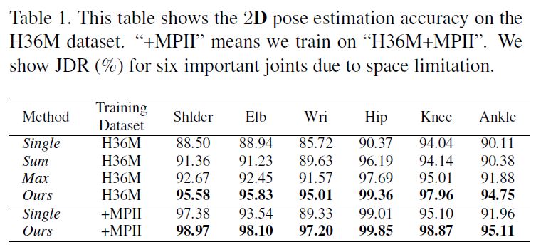
Table 1 shows the results on the most important joints when we train, either only on the H36M dataset, or on a combination of the H36M and MPII datasets.
It compares our approach with the baseline method [31], termed Single, which does not perform cross view feature fusion.
We also compare with two baselines which compute sum or max values over the epipolar line using the camera parameters.
The hyper parameters for training the two methods are kept the same for fair comparison.

Table 1은 우리가 H36M dataset만 또는 H36M과 MPII datasets의 조합을 학습할 때 가장 중요한 joints에 results를 보여준다. 우리의 접근 방식을 cross view feature fusion을 수행하지 않는 Single이라고하는 aseline method [31]과 비교한다. 또한 카메라 매개 변수를 사용하여 epipolar line에 대한 합계 또는 최대 값을 계산하는 두 개의 baselines과 비교한다. 두가지 방법 training에 대한 hyper parameters를 공정한 비교를 위해 같은 보관되어 있다.

Our approach outperforms the baseline Single on all body joints.
The improvement is most significant for the wrist joint, from 85.72% to 95.01%, and from 89.33% to 97.20%, when the model is trained only on “H36M” or on “H36M + MPII”, respectively.
We believe this is because “wrist” is the most frequently occluded joint and cross view fusion fuses the features of other (visible) views to help detect them.
See the third column of Figure 6 for an example.
The right wrist joint is occluded in the current view.
So the detected heatmap has poor quality.
But fusing the features with those of other views generates a better heatmap.
In addition, our approach outperforms the sum and max baselines.
This is because the heatmaps are often noisy especially when occlusion occurs.
Our method trains a fusion network to handle noisy heatmaps so it is more robust than getting sum/max values along epipolar lines.

우리의 접근 방식은 모든 body joints에서 baseline Single을 능가한다.
손목 joint의 경우 85.72%에서 95.01%로, ‘H36M’이나 ‘H36M + MPII’에서만 모델을 훈련할 경우 89.33%에서 97.20%로 개선 효과가 가장 크다.
우리는 “손목”이 가장 자주 가려지는 joint 및 cross view fusion이 다른 (보이는) views의 features을 결합하여 이를 탐지하는 데 도움이 되기 때문이라고 믿는다.
예는 Figure 6의 세 번째 열을 참조.
오른쪽 손목 관절이 현재 view에서는 가려져 있다.
그래서 검출된 heatmap는 품질이 좋지 않다.
그러나 features을 다른 views의 features과 결합하면 더 나은 heatmap이 생성된다.
또한 우리의 접근 방식은 sum 및 max baselines을 능가한다.
특히 occlusion이 발생할 때 heatmaps이 noisy를 일으키는 경우가 많기 때문이다.
우리의 방법은 noisy heatmaps을 처리하기 위해 fusion network를 훈련시켜 epipolar lines을 따라 sum/max 값을 얻는 것보다 더 robust하다.

It is also interesting to see that when we only use the H36M dataset for training, the Single baseline achieves very poor performance.
We believe this is because the limited appearance variation in the training set affects the generalization power of the learned model.
However, our fusion approach suffers less from the lack of training data.
This is probably because the fusion approach requires the features extracted from different views to be consistent following a geometric transformation, which is a strong prior to reduce the risk of overfitting to the training datasets with limited appearance variation.

또한 H36M dataset를 훈련에만 사용할 때 Single baseline이 매우 낮은 성능을 달성한다는 것도 흥미롭다.
우리는 training set의 제한된 외관 변화가 학습된 모델의 generalization power에 영향을 미치기 때문이라고 믿는다.
그러나 우리의 fusion approach는 training data 부족으로 인해 어려움을 덜 겪는다.
이는 fusion approach이 제한된 모양 변화로 training datasets에 과적합될 위험을 줄이는 strong prior인 geometric transformation 후 일관성을 유지하기 위해 서로 다른 views에서 추출 된 features을 요구하기 때문일 수 있다.

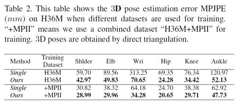
The improved 2D pose estimations in turn help significantly reduce the error in 3D.
We estimate 3D poses by direct triangulation in this experiment.
Table 2 shows the 3D estimation errors on the six important joints.
The error for the wrist joint (which gets the largest improvement in 2D estimation) decreases significantly from 64.18mm to 34.28mm.
The improvement on the ankle joint is also as large as 15mm.
The mean per joint position error over all joints (see (c) and (g) in Table 3) decreases from 36.28mm to 27.90mm when we do not align the estimated 3D pose to the ground truth.

2D pose estimations이 개선되어 3D에서 error를 크게 줄일 수 있다.
우리는 이 실험에서 직접 삼각 측량을 통해 3D poses를 추정한다.
Table 2는 6개의 중요한 joints에 대한 3D estimation errors를 보여준다.
(2D estimation에서 가장 크게 개선된)손목 관절에 대한 error는 64.18mm에서 34.28mm로 크게 감소한다.
발목 관절 개선 또한 15mm까지 크다.
모든 joints에 대한 mean per joint position error(Table 3의 (c) 및 (g))는 우리가 estimated 3D pose를 ground truth에 맞추지 않으면 36.28mm에서 27.90mm으로 감소한다.

6.3. Qualitative Results

In addition to the above numerical results, we also qualitatively investigate in what circumstance our approach will improve the 2D pose estimations over the baseline.
Figure 6 shows four examples.
First, in the fourth example (column), the detected heatmap shows strong responses at both left and right elbows because it is hard to differentiate them for this image.
From the ground truth heatmap (the second row) we can see that the left elbow is the target.
The heatmap warped from other views (fifth row) correctly localizes the left joint.
Fusing the two heatmaps gives better localization accuracy.
Second, the third column of Figure 6 shows the heatmap of the right wrist joint.
Because the joint is occluded by the human body, the detected heatmap is not correct.
But the heatmaps warped from the other three views are correct because it is not occluded there.

위의 수치 결과 외에도, 우리는 우리의 approach가 baseline에 대한 2D pose estimations를 어떤 상황에서 개선할 것인지 질적으로 조사한다.
Figure 6은 네 가지 예를 보여준다.
첫째, 네 번째 예제(열)에서 탐지된 heatmap는 이 이미지에 대해 구별하기 어렵기 때문에 왼쪽과 오른쪽 팔꿈치 모두에서 강력한 반응을 보여줍니다.
ground truth heatmap(두 번째 행)에서 왼쪽 팔꿈치가 target임을 알 수 있다.
다른 views(5번째 행)로부터 뒤틀린 heatmap은 왼쪽 joint의 위치를 올바르게 지정한다.
두 heatmaps을 융합하면 localization accuracy가 향상된다.
둘째, Figure 6의 세 번째 열은 오른쪽 손목 관절의 heatmap을 보여준다.
joint는 human body에 의해 가려지기 때문에 검출된 heatmap이 정확하지 않다.
그러나 다른 세 가지 views로부터 뒤틀린 heatmap은 그것이 그곳에 가려져 있지 않기 때문에 정확하다.

7. Experiments on 3D Pose Estimation

7.1. Implementation Details

In the first iteration of RPSM \((t = 0)\), we divide the space of size 2,000mm around the estimated location of the root joint into 163 bins, and estimate a coarse 3D pose by solving Eq. 2.
We also tried to use a larger number of bins, but the computation time becomes intractable.

RPSM \((t = 0)\)의 첫 번째 반복에서 우리는 루트 조인트의 추정 위치 주위에 2,000mm 크기의 공간을 163개의 빈으로 나누고, Eq. 2를 해결하여 거친 3D 포즈를 추정한다.
우리는 또한 더 많은 수의 빈을 사용하려고 노력했지만, 계산 시간이 다루기 어려워진다.

For the following iterations where \(t ≥ 1\), we divide the space, which is of size \(s_t = \frac{2000}{16×2^{(t−1)}}\) , around each estimated joint location into 2 × 2 × 2 bins.
Note that the space size \(s_t\) of each joint equals to the size of a single bin in the previous iteration.
We use a smaller number of bins here than that of the first iteration, because it can significantly reduce the time for on-the-fly computation of the pairwise potentials.
In our experiments, repeating the above process for ten iterations only takes about 0.4 seconds.
This is very light weight compared to the first iteration which takes about 8 seconds.

\(t ≥ 1\)인 다음 반복의 경우, 우리는 크기 \(s_t = \frac{2000}{16 \times 2^{(t-1)}}\)인 공간을 각각 추정 공동 위치 주위에 2 × 2 x 2 빈으로 나눈다.
각 조인트의 공간 크기 \(s_t\)는 이전 반복에서 단일 빈의 크기와 같다는 점에 유의한다.
여기서는 첫 번째 반복의 빈 수보다 더 적은 수의 빈을 사용하는데, 이는 쌍별 전위를 즉시 계산하는 시간을 크게 줄일 수 있기 때문이다.
우리의 실험에서, 위의 과정을 10번 반복하는 것은 0.4초 밖에 걸리지 않는다.
이것은 약 8초가 걸리는 첫 번째 반복에 비해 매우 가볍습니다.

7.2. Quantitative Results

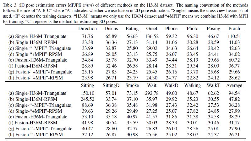
We design eight configurations to investigate different factors of our approach.
Table 3 shows how different factors of our approach decreases the error from 94.54mm to 26.21mm.

우리는 접근 방식의 다양한 요소를 조사하기 위해 8가지 구성을 설계한다.
표 3은 접근 방식의 다른 요소들이 어떻게 오류를 94.54mm에서 26.21mm로 감소시키는지 보여준다.

RPSM vs. Triangulation:
First, RPSM achieves significantly smaller 3D errors than Triangulation when 2D pose estimations are obtained by a relatively weak model.
For instance, by comparing the methods (a) and (b) in Table 3, we can see that, given the same 2D poses, RPSM significantly decreases the error, i.e. from 94.54mm to 47.82mm.
This is attributed to the joint optimization of all nodes and the recursive pose refinement.

첫째, RPSM은 상대적으로 약한 모델에 의해 2D 포즈 추정이 얻어질 때 삼각측량보다 훨씬 작은 3D 오류를 달성한다.
예를 들어, 표 3의 방법 (a)와 (b)를 비교함으로써, 우리는 동일한 2D 포즈로 인해 RPSM이 오류를 94.54mm에서 47.82mm로 크게 감소시킨다는 것을 알 수 있다.
이는 모든 노드의 공동 최적화와 재귀 포즈 미세화 덕분이다.

Second, RPSM provides marginal improvement when 2D pose estimations are already very accurate.
For example, by comparing the methods (g) and (h) in Table 3 where the 2D poses are estimated by our model trained on the combined dataset (“H36M+MPII”), we can see the error decreases slightly from 27.90mm to 26.21mm.
This is because the input 2D poses are already very accurate and direct triangulation gives reasonably good 3D estimations.
But if we focus on some difficult actions such as “sitting”, which gets the largest error among all actions, the improvement resulted from our RPSM approach is still very significant (from 40.47mm to 32.12mm).

둘째, RPSM은 2D 포즈 추정이 이미 매우 정확할 때 한계 개선을 제공한다.
예를 들어, 결합된 데이터 세트(“H36M+MPII”)에서 훈련된 모델에 의해 2D 포즈가 추정되는 표 3의 방법(g)과 (h)을 비교함으로써 오류가 27.90mm에서 26.21mm로 약간 감소하는 것을 알 수 있다.
이는 입력 2D 포즈가 이미 매우 정확하고 직접 삼각 측량이 3D 추정을 합리적으로 잘 제공하기 때문이다.
그러나 모든 작업 중 가장 큰 오류를 얻는 “앉기”와 같은 일부 어려운 작업에 초점을 맞춘다면, RPSM 접근법으로 인한 개선은 여전히 매우 중요하다(40.47mm에서 32.12mm).

In summary, compared to triangulation, RPSM obtains comparable results when the 2D poses are accurate, and significantly better results when the 2D poses are inaccurate which is often the case in practice.

요약하면, RPSM은 삼각측정에 비해 2D 포즈가 정확할 때 비교 가능한 결과를 얻고, 2D 포즈가 부정확할 때 2D 포즈가 훨씬 더 나은 결과를 얻는데, 실제로 종종 그러하다.

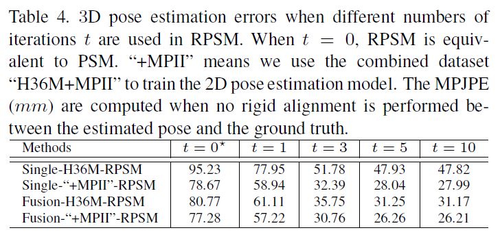
RPSM vs. PSM:
We investigate the effect of the recursive 3D pose refinement.
Table 4 shows the results.
First, the poses estimated by PSM, i.e. RPSM with t = 0, have large errors resulted from coarse space discretization.
Second, RPSM consistently decreases the error as t grows and eventually converges.
For instance, in the first row of Table 4, RPSM decreases the error of PSM from 95.23mm to 47.82mm which validates the effectiveness of the recursive 3D pose refinement of RPSM.

우리는 재귀적인 3D 포즈 미세화의 영향을 조사한다.
표 4는 결과를 보여줍니다.
첫째, PSM에 의해 추정된 포즈, 즉 t = 0인 RPSM은 거친 공간 이산화로 인해 큰 오류를 가지고 있다.
둘째, RPSM은 t가 커지면 오류를 지속적으로 감소시키고 결국 수렴한다.
예를 들어 표 4의 첫 번째 행에서, RPSM은 PSM의 오류를 95.23mm에서 47.82mm로 감소시켜 RPSM의 재귀적 3D 포즈 정제 효과를 검증한다.

Single vs. Fusion:
We now investigate the effect of the cross-view feature fusion on 3D pose estimation accuracy. Table 3 shows the results. First, when we use H36M+MPII datasets (termed as “+MPII”) for training and use triangulation to estimate 3D poses, the average 3D pose error of our fusion model (g) is smaller than the baseline without fusion (c). The improvement is most significant for the most challenging “Sitting” action whose error decreases from 88.69mm to 40.47mm. The improvement should be attributed to the better 2D poses resulted from cross-view feature fusion. We observe consistent improvement for other different setups. For example, compare the methods (a) and (e), or the methods (b) and (f).

이제 크로스 뷰 기능 융합이 3D 포즈 추정 정확도에 미치는 영향을 조사한다. 표 3은 결과를 보여줍니다. 첫째, 훈련에 H36M+MPII 데이터 세트(이하 “+MPI”라 한다)를 사용하고 3D 포즈를 추정하기 위해 삼각측량을 사용할 때, 융합 모델(g)의 평균 3D 포즈 오차는 융합(c)이 없는 기준치보다 작다. 이 개선은 오류가 88.69mm에서 40.47mm로 감소하는 가장 어려운 “앉는” 동작에 가장 중요하다. 개선은 크로스 뷰 기능 융합으로 인한 더 나은 2D 포즈 덕분이어야 한다. 우리는 다른 설정에 대해 일관된 개선을 관찰한다. 예를 들어, 방법(a)과 방법(e) 또는 방법(b)과 방법(f)을 비교합니다.

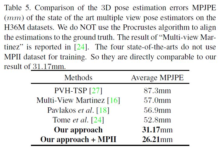
Comparison to the State-of-the-arts:
We also compare our approach to the state-of-the-art methods for multi-view human pose estimation in Table 5.
Our approach outperforms the state-of-the-arts by a large margin.
First, when we train our approach only on the H36M dataset, the MPJPE error is 31.17mm which is already much smaller than the previous state-of-the-art [24] whose error is 52.80mm.
As discussed in the above sections, the improvement should be attributed to the more accurate 2D poses and the recursive refinement of the 3D poses.

우리는 또한 표 5의 다중 뷰 인간 포즈 추정을 위한 최첨단 방법에 대한 우리의 접근 방식을 비교한다.
우리의 접근 방식은 최첨단 기술을 훨씬 능가한다.
첫째, H36M 데이터 세트에 대해서만 접근 방식을 훈련시킬 때 MPJPE 오류는 31.17mm로 오류가 52.80mm인 이전 최첨단 [24]보다 이미 훨씬 작다.
위 절에서 논의한 바와 같이, 개선은 보다 정확한 2D 포즈와 3D 포즈의 재귀적인 정교함에 기인해야 한다.

7.3. Qualitative Results

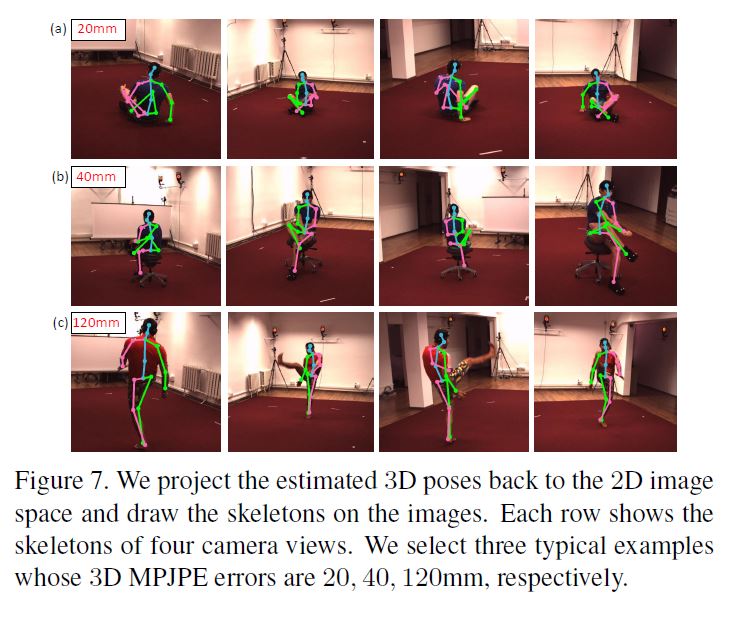
Since it is difficult to demonstrate a 3D pose from all possible view points, we propose to visualize it by projecting it back to the four camera views using the camera parameters and draw the skeletons on the images.
Figure 7 shows three estimation examples.
According to the 3D geometry, if the 2D projections of a 3D joint are accurate for more than two views (including two), the 3D joint estimation is accurate.
For instance, in the first example (first row of Figure 7), the 2D locations of the right hand joint in the first and fourth camera view are accurate.
Based on this, we can infer with high confidence that the estimated 3D location of the right hand joint is accurate.

가능한 모든 뷰 포인트에서 3D 포즈를 시연하는 것은 어렵기 때문에 카메라 매개 변수를 사용하여 4개의 카메라 뷰에 다시 투영하여 시각화하고 이미지에 골격을 그릴 것을 제안한다.
그림 7은 세 가지 추정 예를 보여줍니다.
3D 기하학에 따르면, 3D 이음매의 2D 투영이 2개 이상의 보기(2개 포함)에 대해 정확하다면, 3D 이음매 추정은 정확하다.
예를 들어 첫 번째 예제(그림 7의 첫 번째 행)에서 첫 번째 및 네 번째 카메라 뷰에서 오른쪽 조인트의 2D 위치가 정확합니다.
이를 바탕으로, 우리는 오른손 관절의 추정 3D 위치가 정확하다는 높은 확신을 가지고 추론할 수 있다.

In the first example (row), although the right hand joint is occluded by the human body in the second view (column), our approach still accurately recovers its 3D location due to the cross view feature fusion.
Actually, most leg joints are also occluded in the first and third views but the corresponding 3D joints are estimated correctly.

첫 번째 예(행)에서 오른쪽 관절은 두 번째 보기(열)에서 인체에 의해 가려지지만, 우리의 접근 방식은 여전히 교차 보기 기능 융합으로 인해 3D 위치를 정확하게 복구한다.
실제로 대부분의 다리 관절도 첫 번째 보기와 세 번째 보기에서는 가려지지만 해당 3D 관절은 정확하게 추정됩니다.

The second example gets a larger error of 40mm because the left hand joint is not accurately detected.
This is because the joint is occluded in too many (three) views but only visible in a single view.
Cross-view feature fusion contributes little in this case.
For most of the testing images, the 3D MPJPE errors are between 20mm to 40mm.

두 번째 예에서는 좌측 조인트가 정확하게 감지되지 않기 때문에 40mm의 더 큰 오차가 발생합니다.
그 이유는 조인트가 너무 많은(3개) 보기에 가려져 있지만 단일 보기에만 표시되기 때문입니다.
이 경우 크로스 뷰 기능 융합은 거의 도움이 되지 않습니다.
대부분의 테스트 이미지의 경우 3D MPJPE 오류는 20mm에서 40mm 사이입니다.

There are few cases (about 0.05%) where the error is as large as 120mm. This is usually when “double counting” happens.
We visualize one such example in the last row of Figure 7.
Because this particular pose of the right leg was rarely seen during training, the detections of the right leg joints fall on the left leg regions consistently for all views.
In this case, the warped heatmaps corresponding to the right leg joints will also fall on the left leg regions thus cannot drag the right leg joints to the correct positions.

120mm만큼 오차가 큰 경우는 거의 없습니다(약 0.05%). 이것은 보통 “이중 계수”가 일어날 때 일어난다.
그림 7의 마지막 행에서 이러한 예 하나를 시각화합니다.
훈련 중에는 오른쪽 다리의 이러한 특정한 자세를 거의 볼 수 없었기 때문에, 오른쪽 다리 관절의 탐지는 모든 시야에 대해 일관되게 왼쪽 다리 부위에 떨어진다.
이 경우 오른쪽 다리 관절에 해당하는 뒤틀린 열 지도도 왼쪽 다리 부위에 떨어지기 때문에 오른쪽 다리 관절이 올바른 위치로 끌려갈 수 없다.

7.4. Generalization to the Total Capture Dataset

We conduct experiments on the Total Capture dataset to validate the general applicability of our approach.
Our model is trained only on the Total Capture dataset.
Table 6 shows the results. “Single-RPSM” means we do NOT perform cross-view feature fusion and use RPSM for recovering 3D poses.
First, our approach decreases the error of the previous best model [26] by about 17%.
Second, the improvement is larger for the hard cases such as “FS3”. The results are consistent with those on the H36M dataset. Third, by comparing the approaches of “Single-RPSM” and “Fusion-RPSM”, we can see that fusing the features of different views improves the final 3D estimation accuracy significantly. In particular, the improvement is consistent for all different subsets.

우리는 접근 방식의 일반적인 적용 가능성을 검증하기 위해 Total Capture 데이터 세트에 대한 실험을 수행한다.
우리의 모델은 Total Capture 데이터 세트에서만 훈련된다.
표 6은 결과를 보여줍니다. “Single-RPSM”은 크로스 뷰 기능 융합을 수행하지 않으며 3D 포즈 복구를 위해 RPSM을 사용합니다.
첫째, 우리의 접근 방식은 이전의 최고 모델[26]의 오차를 약 17% 감소시킨다.
둘째, “FS3”와 같은 하드 케이스에 대한 개선 폭이 더 크다. 결과는 H36M 데이터 세트의 결과와 일치한다. 셋째, “Single-RPSM”과 “Fusion-RPSM”의 접근 방식을 비교함으로써 서로 다른 보기의 특징을 융합하면 최종 3D 추정 정확도가 크게 향상됨을 알 수 있다. 특히, 개선은 모든 다른 부분 집합에 대해 일관적입니다.

7.5. Generalization to New Camera Setups

We conduct experiments on the H36M dataset using NO pose annotations.
The single view pose estimator [31] is trained on the MPII dataset.
If we directly apply this model to the test set of H36M and estimate the 3D pose by RPSM, the MPJPE error is about 109mm.
If we retrain this model (without the fusion layer) using the harvested pseudo labels, the error decreases to 61mm.
If we train our fusion model with the pseudo labels described above, the error decreases to 43mm which is already smaller than the previous supervised state-of-the-arts.
The experimental results validate the feasibility of applying our model to new environments without any manual label.

NO pose annotations을 사용하여 H36M dataset에 대한 실험을 수행한다.
single view pose estimator[31]는 MPII dataset에 대해 훈련된다.
이 모델을 H36M의 test set에 직접 적용하고 RPSM으로 3D pose를 추정하면, MPJPE error는 약 109mm이다.
수확된 pseudo labels을 사용하여 (fusion layer 없는)이 모델을 재교육하면 error가 61mm로 감소한다.
위에서 설명한 pseudo labels로 fusion model을 훈련하면 error가 43mm로 줄어 이미 이전의 supervised state-of-the-arts보다 작다.
실험 결과는 수동 label 없이 우리의 모델을 새로운 환경에 적용할 수 있는 가능성을 검증한다.

8. Conclusion

We propose an approach to estimate 3D human poses from multiple calibrated cameras.
The first contribution is a CNN based multi-view feature fusion approach which significantly improves the 2D pose estimation accuracy.
The second contribution is a recursive pictorial structure model to estimate 3D poses from the multi-view 2D poses.
It improves over the PSM by a large margin.
The two contributions are independent and each can be combined with the existing methods.

우리는 여러 대의 보정 된 카메라에서 3D 인간 포즈를 추정하는 접근 방식을 제안합니다.
첫 번째 기여는 2D 포즈 추정 정확도를 크게 향상시키는 CNN 기반 멀티 뷰 기능 융합 접근 방식입니다.
두 번째 기여도는 다중 뷰 2D 포즈에서 3D 포즈를 추정하는 재귀 적 그림 구조 모델입니다.
PSM보다 큰 차이가 있습니다.
두 가지 기여는 독립적이며 각각 기존 방법과 결합 할 수 있습니다.