IEEE 2020 paper

• ABSTRACT
• INDEX TERMS
• I. INTRODUCTION
  • A. RELATED WORKS
  • B. BASIC STEPS IN POSE ESTIMATION
• II. POSE ESTIMATION PRELIMINARY
  • A. SINGLE/MULTI-PERSON POSE ESTIMATION
  • B. APPROACHES IN POSE ESTIMATION
  • C. APPLICATIONS OF POSE ESTIMATION
  • D. CHALLENGES FACING
• III. MAIN COMPONENTS OF POSE ESTIMATION
  • A. BACKBONE ARCHITECTURE
  • B. LOSS FUNCTIONS
  • C. DATASET
  • D. COMMON EVALUATION METRICS
• IV. MAJOR RESEARCHES IN HUMAN POSE ESTIMATION
  • A. DeepPose
  • B. ConvNet POSE: EFFICIENT OBJECT LOCALIZATION USING CONVOLUTIONAL NETWORKS
  • C. CPM: CONVOLUTIONAL POSE MACHINES
  • D. STACKED HOURGLASS NETWORKS FOR HUMAN POSE ESTIMATION
  • E. DeeperCut: A DEEPER, STRONGER, AND FASTER MULTI-PERSON POSE ESTIMATION MODEL
  • F. IEF: HUMAN POSE ESTIMATION WITH ITERATIVE ERROR FEEDBACK
  • G. REALTIME MULTI-PERSON2D POSE ESTIMATION USING PART AFFINITY FIELDS
  • H. CPN: CASCADED PYRAMID NETWORK FOR MULTI-PERSON POSE ESTIMATION
  • I. SIMPLE BASELINES FOR HUMAN POSE ESTIMATION AND TRACKING
  • J. HRNet: DEEP HIGH-RESOLUTION REPRESENTATION LEARNING FOR HUMAN POSE ESTIMATION
  • K. CFA: CASCADE FEATURE AGGREGATION FOR HUMAN POSE ESTIMATION
  • L. OccNet: HUMAN POSE ESTIMATION FOR REAL-WORLD CROWDED SCENARIOS
  • M. DarkPose: DISTRIBUTION-AWARE COORDINATE REPRESENTATION FOR HUMAN POSE ESTIMATION
• V. SUMMARY AND DISCUSSION
• VI. CONCLUSION

ABSTRACT

Human pose estimation localizes body keypoints to accurately recognizing the postures of individuals given an image.
This step is a crucial prerequisite to multiple tasks of computer vision which include human action recognition, human tracking, human-computer interaction, gaming, sign languages, and video surveillance.
Therefore, we present this survey article to fill the knowledge gap and shed light on the researches of 2D human pose estimation.
A brief introduction is followed by classifying it as a single or multi-person pose estimation based on the number of people needed to be tracked.
Then gradually the approaches used in human pose estimation are described before listing some applications and also flaws facing in pose estimation.
Following that, a center of attention is given on briefly discussing researches with a significant effect on human pose estimation and examine the novelty, motivation, architecture, the procedures (working principles) of each model together with its practical application and drawbacks, datasets implemented, as well as the evaluation metrics used to evaluate the model.
This review is presented as a baseline for newcomers and guides researchers to discover new models by observing the procedure and architecture flaws of existing researches.

Human pose estimation은 이미지가 주어지고 개인의 자세를 정확하게 인식하기 위해 body keypoints를 위치시킨다.
이 단계는 human action recognition, human tracking, human-computer interaction, gaming, sign languages, 그리고 video surveillance를 포함하는 컴퓨터 비전의 여러 작업에 대한 중요한 전제 조건이다.
따라서, 우리는 지식 격차를 메우기 위해 이 survey article를 제시하고 2D human pose estimation의 연구를 조명한다.
간단한 소개에 이어 추적해야 할 사람수를 기준으로 single-person pose estimation 또는 multi-person pose estimation으로 분류한다.
이 후 일부 applications과 pose estimatio이 직면한 결함을 설명하기 전에 human pose estimation에 사용되는 접근법을 설명한다. 그 후, human pose estimation에 상당한 영향을 미치는 연구를 간략하게 논의하고 각 모델의 novelty, motivation, architecture procedures(작업 원리)와 application 및 단점, 구현된 datasets, 그리고 model을 평가하는데 사용된 evaluation metrics를 함께 검토하는 데 집중한다.
이 review는 newcomers의 baseline으로 제시하며, 기존 연구의 절차와 architecture 결함을 관찰하여 연구자가 새로운 모델을 발견하도록 안내한다.

INDEX TERMS

Human pose estimation, pose estimation and action recognition, pose estimation survey, single and multi-person pose estimation.

I. INTRODUCTION

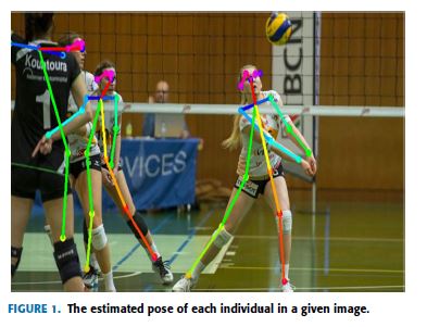
Human pose estimation is one of the challenging fields of study in computer vision which aims in determining the position or spatial location of body keypoints (parts/joints) of a person from a given image or video [1], [2], as shown in Fig.1.
Thus, pose estimation obtains the pose of an articulated human body, which consists of joints and rigid parts using image-based observations [3].
Human pose estimation refers to the process of inferring poses in an image and these estimations are performed in either 3D or 2D [4].
To solve this problem, several approaches in the literature have been proposed.
Early works introduced the classical approaches to articulated human pose estimation called the pictorial structures [5]-[8].
In these models, the spatial correlations of the body parts are demonstrated as a tree-structured graphical model and they are very successful when the limbs are visible however faced problems when the tree-structured fails capturing the correlation between variables.
Hand-crafted features such as edges, contours, the histogram of oriented gradients (HOG) features, and color histograms have also been used in early works for human pose estimation [9]-[13].
These models have shown bad generalization performance which faced problems in detecting the accurate location of the body parts.

Human pose estimation은 Fig.1에 표시된 것처럼 주어진 image 또는 video에서 사람의 body keypoints (parts/joints)의 position 또는 spatial location를 결정하는 것을 목표로 하는 computer vision 연구의 어려운 분야 중 하나이다. [1], [2]
따라서 pose estimation은 image-based 관찰을 사용하여 joints과 rigid parts로 구성된 articulated human body의 pose를 얻는다 [3].
Human pose estimation은 image에서 poses를 유추(infer)하는 과정을 의미하며 이러한 estimations은 3D 또는 2D에서 수행된다 [4].
이 문제를 해결하기 위해, 문헌에서 몇 가지 접근법이 제안되었다.
초기 works들은 pictorial structures라고 불리는 articulated human pose estimation에 대한 고전적인 접근 방식을 도입했다 [5]-[8].
이러한 모델에서 body parts의 spatial 상관 관계는 tree-structured graphical model로 입증되며, 팔다리(limbs)가 보일 때 매우 성공적이지만 tree-structured가 variables 간의 상관 관계를 capturing하지 못할 때 문제에 직면한다.
edges, contours(윤곽선), the histogram of oriented gradients (HOG) features 와 color histograms과 같은 Hand-crafted features도 초기 works에는 human pose estimation을 위해 사용되었다 [9]-[13].
이러한 모델은 body parts의 정확한 location를 감지하는 데 문제가 발생한 좋지 않은 generalization performance를 보여주었다.

Contributions:
Solving the problems and challenges related to human pose estimation has been advanced and progressed remarkably with the help of deep learning and publicly available datasets.
This survey provides a summary of these works comprehending up to date information and points the future research directions.
Like some remarkable surveys [14]-[18], this paper also provides a general concept of human pose estimation.
It can be used as a guideline for people who are new to this concept and helps them to define noble models by combining the network structures of the existing models.
Additionally, it helps researchers to compare their work with significant models based on deep learning.
Besides, here are some specific main contributions of this review:

Contributions:
human pose estimation과 관련된 challenges 및 문제 해결은 deep learning과 publicly available datasets의 도움을 받아 매우 진전되었다.
본 survey는 이러한 연구의 요약본으로 최신 정보를 파악하고 향후 연구 방향을 제시한다.
일부 주목할 만한 surveys[14]-[18]와 마찬가지로, 본 논문에서는 human pose estimation의 일반적인 개념도 제공한다.
이 개념을 처음 접하는 사람들을 위한 guideline으로 활용할 수 있으며, 기존 모델의 network 구조를 결합해 noble models을 정의할 수 있도록 돕는다.
또한, 그것은 연구자들이 deep learning을 기반으로 한 중요한 models과 그들의 연구를 비교할 수 있도록 돕는다.
또한, 다음은 이 review의 몇 가지 주요 contributions이다 :

• Provides a summary of preferred backbone architectures and loss functions used in addition to the overview of evaluation metrics implied and datasets employed.
• Provides an overview of recent models on 2D human pose estimation
• Limitations of each model’s work and open issues are presented

• 암시된 evaluation metrics와 채택된 datasets의 개요와 함께 사용되는 기본 backbone architectures 와 loss functions의 summary를 제공.
• 2D human pose estimation에 대한 최신 모델의 개요를 제공합니다.
• 모델별 work 및 open issues의 한계 제시

A. RELATED WORKS

Other survey papers related to pose estimation have been released in the past years.
For example, two survey papers [14], [15] published in 2016 have extensively surveyed models on human pose estimation which did not implement deep learning-based approaches.
Then [16] presented a survey of deep learning, pose estimation, and application of deep learning for computer vision.
A review on hand pose estimation is presented by [19] whereas [20] provided a survey on head pose estimation.

pose estimation과 관련된 다른 survey papers은 지난 몇 년 동안 발표되었다.
예를 들어, 2016년에 발표된 두 개의 survey papers [14], [15]은 deep learning-based approaches을 구현하지 않은 human pose estimation에 대한 models을 광범위하게 조사했다.
그리고 [16]은 computer vision에 대한 deep learning, pose estimation 및 application에 대한 survey를 제시하였다.
hand pose estimation에 대한 review [19]는 에 의해 제시되며 [20]은 head pose estimation에 대한 survey를 제공한다.

One of the recent surveys on 2D human pose estimation based on deep learning is [17].
This review started by categorizing pose estimation as a single person and multi-person pipeline and in each category created sub-categories.
Another survey on deep-learning-based pose estimation has just come out [18] on both 2D and 3D pose estimation.
2D human pose estimation is categorized as [17] while 3D human pose estimation is categorized as model-free and model-based and the approaches are discussed based on these categories in both cases.

2D human pose estimation based on deep learning에 대한 최근 surveys 중 하나는 [17]이다. 이 review는 pose estimation을 single person와 multi-person pipeline으로 분류하고 생성된 각 범주에서 하위 범주로 분류함으로써 시작되었다. deep-learning-based pose estimation에 대한 그리고 2D 및 3D pose estimation에 대한 또 다른 survey[18]가 최근 나왔다. 2D human pose estimation은 [17]로 분류되는 반면, 33D human pose estimation은 model-free 과 model-based로 분류되며, 두 경우 모두 이러한 범주에 기초하여 접근법이 논의된다.

This survey paper presents different deep learning-based 2D human pose estimation models.
The backbone architecture used, loss functions, the datasets used, as well as evaluation metrics implied are discussed and evaluated.
The main objective of this paper is to provide a detailed analysis of mostly known effective models used, provide readers with various opportunities in mixing architecture of different models so that to come up with better human pose estimation models using better evaluation metrics or efficient backbone architecture.

본 survey paper는 다양한 deep learning-based 2D human pose estimation models을 제시한다.
사용된 backbone architecture, loss functions, 사용된 datasets 및 암시된 evaluation metrics이 논의되고 평가된다.
본 논문의 주요 목표는 주로 사용되는 것으로 알려진 effective models에 대한 상세한 분석을 제공하고, 독자에게 다양한 모델의 architecture를 혼합하는 다양한 기회를 제공하여 더 나은 evaluation metrics 또는 효율적인 backbone architecture를 사용하는 더 나은 human pose estimation models을 고안하는 것이다.

B. BASIC STEPS IN POSE ESTIMATION

The main process of human pose estimation is boiled into two basic steps:
i) localizing human body joints/keypoints and;
ii) grouping those joints into valid human pose configuration [7], [8].
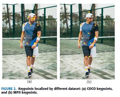
In the first step, the main focus is on finding the location of each keypoints of human beings as displayed in Fig.2. E.g. Head, shoulder, arm, hand, knee, ankle.

human pose estimation의 주요 과정은 두 가지 기본 단계로 나뉜다.
i) human body joints/keypoints 위치 파악 및
ii) 이 joints를 유효한 인체 포즈 구성으로 그룹화[7], [8]

In the first step, the main focus is on finding the location of each keypoints of human beings as displayed in Fig.2. E.g. Head, shoulder, arm, hand, knee, ankle.

Collecting and identifying these joints can be done through any of the different popular dataset formats; such that the way keypoints are stored in the selected dataset.
As shown in Fig.2, different platforms can result in different dataset output formats for the same image of body joints.
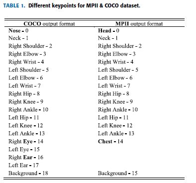
For instance, COCO [21], dataset provide 17 body joints whereas MPII [22] provides 14 body joints.
Table 1 displays the outputs dataset for the two platforms.

첫 번째 단계에서 주요 초점은 머리, 어깨, 팔, 손, 무릎, 발목과 같은 Fig.2에 표시된 인간의 각 keypoints의 location을 끝내는 것이다.
이러한 joints를 수집하고 식별하는 것은 ;keypoints가 선택한 dataset에 저장되는 방법 등과 같이; 널리 사용되는 여러 dataset formats을을 통해 수행할 수 있다.
Fig.2에서 보듯이, 다른 플랫폼들은 동일한 body joints 이미지에 대해 다른 dataset output formats을 초래할 수 있다.
예를 들어, COCO [21] dataset는 17개의 body joints를 제공하는 반면, MPII [22]는 14개의 body joints를 제공한다.
Table 1에는 두 플랫폼에 대한 outputs dataset를 표시하고 있다.

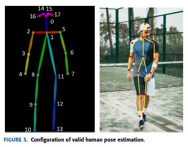
The second step is grouping those joints into valid human pose configuration which determines the pairwise terms between body parts as seen in Fig.3.
Different techniques have been applied in joining the keypoint candidates [23], [24].

두 번째 단계는 Fig.3에서 보는 바와 같이 body parts 사이의 pairwise terms을 결정하는 유효한 인체 자세 구성으로 이 joints을 그룹화하는 것이다.
keypoint 후보군에 합류하는 데는 다양한 기술이 적용되었다 [23], [24].

The rest of this paper is organized as follows.
Section II describes the category of pose estimation based on the number of people needed to track, approaches used in pose estimation, application of pose estimation, and flaws/challenges in pose estimation.
Section III started by the introduction of backbone architectures used, the loss functions, dataset implied, and finally common evaluation metrics used to evaluate models.
In section IV, a detailed discussion of each model’s network procedures is discussed.
Section V summarizes the models in short as a table and opens discussion based on presented in this article and finally section VI concludes the paper’s works.

본 논문의 나머지 부분은 다음과 같이 구성되어 있다.
Section II에서는 tracking에 필요한 pose estimation based on the number of people의 category, pose estimation에 사용된 approaches, pose estimation의 application, pose estimation의 flaws/challenges를 설명한다.
Section III는 사용된 backbone architectures, loss functions, 암시된 dataset, 마지막으로 models 평가에 사용되는 공통 evaluation metrics의 도입으로 시작되었다.
Section IV에서는 각 model’s network procedures에 대한 자세한 discussion이 논의된다.
Section V는 models을 간략하게 table로 요약하고 이 글에 제시된 내용을 기반으로 discussion을 열고
마지막으로 Section VI는 본 논문의 작업을 마무리한다.

II. POSE ESTIMATION PRELIMINARY

This section discusses the general classification of pose estimation based on the number of people to track, introduce the most popular approaches, application of pose estimation, and finally, the challenges that still require new as well as innovative approaches.

이 section에서는 tracking을 위한 pose estimation based on the number of people의 일반적인 분류, 가장 인기 있는 approaches 소개, pose estimation의 application, 마지막으로 여전히 새롭고 혁신적인 approaches이 필요한 challenges에 대해 설명다.

A. SINGLE/MULTI-PERSON POSE ESTIMATION

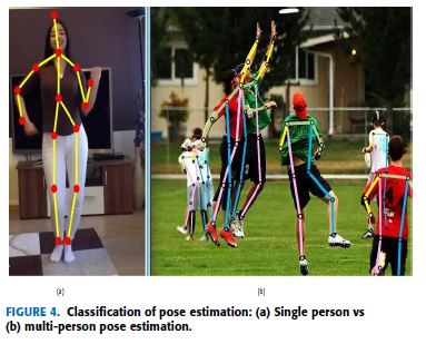
Based on the number of individuals being estimated given an image, pose estimation is classified as single-person and/or multi-person pose estimation.
Single-person pose estimation is much easier compared to multi-person, to estimate pose for a single person from a given image which may contain (usually does) more than a single person.
On the other hand, multi-person pose estimation determines the pose of all individuals available in the image [25].
Fig.4 shows the approach of a single person and multi-person pose estimation applied in the given images.

Based on the number of individuals being estimated given an image, pose estimation은 single-person and/or multi-person pose estimation으로 분류된다.
Single-person pose estimation은 multi-person에 비해 훨씬 쉬우며, single person이상이 포함된 image에서 single person의 pose를 estimate한다. 반면에, multi-person pose estimation은 이미지에서 사용 가능한 모든 개인의 pose를 결정한다 [25].
Fig.4는 주어진 영상에 적용된 single person 과 multi-person pose estimation의 approach를 보여준다.

The use and introduction of deep learning-based architectures [36]-[39] and the availability of large-scale datasets such as MPII human pose dataset [22], COCO [21], and LSP [40] both single and multi-person pose estimation problems have lately been getting attention more and more.

deep learning-based architectures [36]-[39]의 사용 및 도입과 MPII human pose dataset [22], COCO[21], LSP[40]와 같은 large-scale datasets의 가용성이 최근 single 및 multi-person pose estimation 문제에 점점 더 주목을 받고 있다.

B. APPROACHES IN POSE ESTIMATION

Two common approaches are employed in estimating the poses of individuals in a given image.
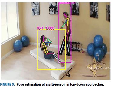
1) Top-down approaches, the processing is done from low to high resolutions, follow the detection of the individual instances in the image first using a bounding box object detector and then focus on determining their poses next [26], [27], [29], as shown in Fig.5.

given image에서 개인의 poses를 추정하는 데 두 가지 일반적인 approaches가 사용된다.
1) Top-down approaches은 low resolutions에서 high resolutions로 처리되며, 먼저 bounding box object detector를 사용하여 image의 개별 instances 탐지를 수행한 후 Fig.5와 같이 다음의 poses를 결정하는 데 초점을 맞춘다 [26], [27], [29].

These approaches always suffer from early commitment, which means if the detection of individuals fails, there is no possibility of recovering.
Also, it is vulnerable when multiple individuals are nearby.
Furthermore, the computational cost depends on the number of people in the image, the more the people the more the computational cost.
Hence, the run-time of these approaches is directly proportional to the number of people: means for every detection, a single-person pose estimator is run.

이러한 approaches는 early commitment로 인해 어려움을 겪는데, 이는 개인 탐지가 실패할 경우 recovering될 가능성이 없다는 것을 의미한다.(= detect를 못하면 pose estimation을 전혀 할수 없음)
또한 여러 사람이 근처에 있을 때 취약하다.
더욱이, 계산 비용은 image의 사람 수에 따라 달라지며, 사람이 많을수록 계산 비용이 증가한다.
따라서 이러한 approaches의 run-time은 사람 수에 정비례한다: 모든 탐지에 대해 평균은 single-person pose estimator가 실행된다.

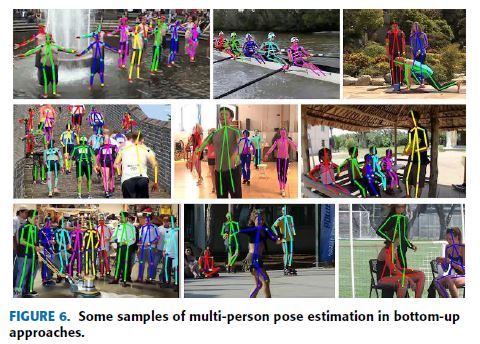
2) The bottom-up approaches [31]-[34] processing is done from high to low resolutions.
It starts by localizing identity-free semantic entities and then grouping them into person instance.
Bottom-up approaches overcame early commitment and showed detached run-time complexity from the number of people in the image as shown in Fig.6.
In addition to that, some researches using bottom-up approaches use the global contextual cues from other body parts and other people.
However, bottom-up approaches face challenges in grouping body parts when there is a large overlap between people.

2) bottom-up approaches [31]-[34] processing은 high resolutions에서 low resolutions으로 수행된다. 그것은 identity-free semantic entities를 지역화한 다음 그것들을 person instance로 그룹화하는 것으로 시작한다. ttom-up approaches은 early commitment을 극복하고 Fig.6에 표시된 것처럼 image의 사람 수로부터 분리된 run-time 복잡성을 보여주었다. 또한 bottom-up approaches를 사용한 일부 연구는 다른 body parts 및 다른 사람의 global contextual 단서를 사용한다. 그러나 bottom-up approaches은 사람 간에 큰 겹침이 있을 때 body parts를 그룹화하는 데 있어 어려움에 직면한다.

C. APPLICATIONS OF POSE ESTIMATION

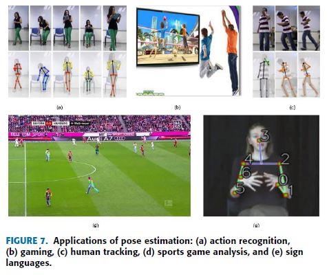
Earlier human pose estimation application areas such as action recognition, human tracking, animation, and gaming [41], [42] are mentioned.
Video surveillance, assisted living, and advanced driver assistance systems (ADAS) [43], [44] are also included.
Furthermore, it may also provide game analysis in sports by describing the players’ movement [45].
Pose estimation is also applicable in Sign languages to help disabled people.
Some of the most common current applications of pose estimation are depicted in Fig.7.

이에 앞서 action recognition, human tracking, animation, gaming와 같은 human pose estimation 적용분야[41], [42]가 언급되어 있다.
Video surveillance, assisted living, advanced driver assistance systems (ADAS)가 [43], [44]에 포함되어 있다.
게다가, 그것은 또한 players’ movement [45]를 설명함으로써 스포츠에 게임 분석을 제공할 수 있다.
또한 Pose estimation은 Sign languages로 장애인들을 돕는 것에도 적용가능하다. 어떤 pose estimation의 가장 흔한 현재 적용은 Fig.7를 참고.

D. CHALLENGES FACING

Principally every state-of-the-art (SOTA) pose estimation model includes a component that detects body joints or estimates their position and making pairwise terms between body part hypotheses which assist categorizing the pairwise terms into valid human pose configurations.
In doing so, some challenges are faced.
Such as position and scale of each person in the image; barely visible joints; interactions between people, which brings complex spatial interference due to clothing, lighting changes, contact, occlusion of individual parts by clothes, backgrounds, and limb articulations which makes the association of parts difficult.
As the cost of 3D depth-sensing camera decreases and the machine learning algorithms to process the datasets of such technologies improve, we believe that it would bring new approaches to solve current challenges.

기본적으로 모든 최신 (SOTA) pose estimation model에는 body joints을 detect하거나 position을 estimate하는 구성 요소(component) 그리고 pairwise terms를 valid human pose configurations로 분류하는 데 도움이 되는 body part hypotheses간에 pairwise terms을 만드는것을 포함한다. 그렇게함으로써 몇 가지 도전에 직면하게된다. image에서 각 사람의 position와 scale과 같은; 간신히 보이는 joints, 옷 때문에 복잡한 공간 간섭을 가져오는 사람들간의 상호작용, 조명 변화, 접촉, 옷에 의한 ndividual parts의 occlusion, 배경, 팔다리 articulations이 parts 연결을 어렵게 만든다. 3D depth-sensing camera의 비용이 감소하고 이러한 기술의 datasets를 처리하는 machine learning algorithms이 개선됨에 따라 현재 문제를 해결하기위한 새로운 approaches를 가져올 것이라고 믿는다.

III. MAIN COMPONENTS OF POSE ESTIMATION

Before diving into the details of each research model, better to explore first the main components of the pose estimation research’s fundamentals such as backbone architecture, pose loss functions inhabited, the dataset used, and also evaluation metrics applied.

각 연구 model의 세부 정보를 살펴보기 전에, 먼저 backbone architecture, 사용되는 pose loss functions, 사용된 dataset, 적용된 evaluation metrics과 같은 pose estimatio 연구의 기초의 main components를 탐색하는 것이 좋다.

A. BACKBONE ARCHITECTURE

DeepPose [46] is the first significant research article that applied deep learning to human pose estimation.
The authors have implemented the network architecture of AlexNet [37] as backbone architecture which consists of five convolution layers, two fully connected layers, and a softmax classifier.
After the introduction of AlexNet, other machine learning algorithms such as R-CNN [47], Fast R-CNN [48], FPN [49], Faster R-CNN [50] and Mask R-CNN [39] have been used as backbone architecture for other human pose estimation researches [51], [32] and [52].
The second most popular backbone architecture is VGG [36] which has been used in [29], [34].
Although AlexNet and VGG have been in use for a while, most of the recent researches in human pose estimation [26], [27], [31], [32], [35], [53], have been using ResNet [38] as a backbone architecture.

DeepPose[46]는 deep learning을 human pose estimation에 최초로 적용한 중요 연구이다.
저자들은 다섯 개의 convolution layers, 두 개의 fully connected layers, 그리고 softmax classifier로 구성된 backbone architecture로서 AlexNet [37]의 network architecture를 구현했다.
AlexNet의 도입 이후, R-CNN[47], Fast R-CNN[48], FPN[49], Fast R-CNN[50] 및 Mask R-CNN[39]과 같은 다른 머신 러닝 알고리즘은 다른 human pose estimation 연구[51], [32], [52]의 backbone architecture로 사용되어 왔다.
두 번째로 널리 사용되는 backbone architecture는 [29], [34]에서 사용된 VGG[36]이다.
비록 AlexNet과 VGG가 한동안 사용되어 왔지만, human pose estimation [26], [27], [31], [32], [35], [53]의 최근 연구는 ResNet[38]을 backbone architecture로 사용하고 있다.

B. LOSS FUNCTIONS

As one part of machine learning, human pose estimation models learn by loss functions.
Loss functions evaluate how well a specific algorithm models the given dataset.
It reduces the error in the prediction process [54], [55].
Largely three kinds of loss functions applied in human pose estimation models, namely, Mean Absolute Error (MAE), Mean Squared Error (MSE), and Cross-Entropy loss.

머신 러닝의 한 부분으로서, human pose estimation models은 loss functions를 통해 학습한다.
Loss functions는 특정 알고리즘이 주어진 데dataset를 얼마나 잘 모델링하는지 평가한다.
이렇게 하면 prediction process [54], [55]의 오차가 줄어든다.
human pose estimation models에 적용되는 loss functions의 종류는 크게 세 가지로, 즉, Mean Absolute Error (MAE), Mean Squared Error (MSE), Cross-Entropy loss이다.

MAE or L1 loss function is calculated as the average of sums of all absolute differences between true and predicted values.
L1 loss function does not consider the direction, but only measures the magnitude of the error.
The L1 loss function is not sensitive to outliers thus it is robust.
But it is very hard to regress precisely which brings complexity for machine learning [56]. \[L_1 = \frac{1}{n} \sum^n_{i=1} \vert y_i - f(x_i)\vert , \; \; \; (1)\]

MAE 또는 L1 loss function는 true 값과 예측 값 사이의 모든 절대 차이 합계의 평균으로 계산된다.
L1 loss function는 방향을 고려하지 않고 오차의 크기만 측정한다.
L1 loss function는 특이치에 민감하지 않으므로 robust하다.
그러나 machine learning에 복잡성을 가져오는 정확한 regress은 매우 어렵다 [56].

MSE also called L2 loss or Quadratic loss function is calculated as the average of the squared differences between true and predicted values.
Like L1 loss, the L2 loss function measures the magnitude of error without considering the direction.
L2 loss function provides an easier way to calculate gradients due to its mathematical properties.
But, the L2 loss function is very sensitive to outliers, unlike L1 because of its usage of squaring when predicted values and true values are very far away occasionally [56]. \[L_2 = \frac{1}{n} \sum^n_{i=1} (y_i - f(x_i))^2\]

L2 loss 또는 Quadratic loss function라고도 하는 MSE는 true 값과 예측 값 사이의 제곱 차이의 평균으로 계산된다.
L1 loss과 마찬가지로, L2 loss function는 방향을 고려하지 않고 오차 크기를 측정한다.
L2 loss function는 수학적 특성으로 인해 gradients를 계산하기 더 쉬운 방법을 제공한다.
그러나, L2 loss function는 L1과 달리 특이치에 매우 민감한데, 이는 예측 값과 true 값이 때때로 매우 멀리 있을 때 제곱을 사용하기 때문이다 [56].

In Cross-Entropy loss (Negative Log-Likelihood or Log loss), each predicted probability is compared to the actual class output value (0 or 1) and a score is calculated that penalizes the probability based on the distance from the expected value [54].
The penalty is logarithmic, offering a small score for small differences (0.1 or 0.2) and an enormous score for a large difference (0.9 or 1.0) [54].
This means an algorithm with smaller Cross-Entropy loss is preferable, and if it has 0.0 Log loss, then it predicts perfect probability. \[\text{Log}_{loss} = -(y_i \text{log}(f(x_i)) + (1-y_i)\text{log}(1-f(x_i))) \; \; \; (3)\]

Cross-Entropy loss (Negative Log-Likelihood or Log loss)에서 각 예측 확률을 실제 클래스 출력 값(0 또는 1)과 비교하고 예상 값으로부터의 거리에 기초한 확률에 penalty를 주는 점수로 계산합니다 [54].
penalty는 로그로 작은 차이(0.1 또는 0.2)에 작은 점수(0.9 또는 1.0)를 제공하고 큰 차이(0.9 또는 1.0)에 큰 점수를 제공합니다 [54].
이는 더 작은 Cross-Entropy loss를 가지는 알고리즘이 바람직하다는 것을 의미하며, 0.0 Log loss이 있으면 완벽한 확률을 예측한다.

C. DATASET

Researchers in human pose estimation have been mainly using the following four datasets which are freely available to the public: FLIC, LSP, MPII Human Pose, and COCO.
Less known datasets such as Pascal VOC [57], SURREAL [58] for single-person in both 2D and 3D pose estimation, HumanEva, Human3.6 dataset, CrowdPose [59], and JTA [60] have also been used in human pose estimation.

human pose estimation의 연구자들은 대중이 자유롭게 사용할 수 있는 다음과 같은 4개의 datasets를 주로 사용해 왔다: FLIC, LSP, MPII Human Pose, COCO.
, 2D 및 3D pose estimation 모두에서 single-person을 위한 Pascal VOC [57], SERPRIC [58], 그리고 HumanEva, Human 3.6 dataset, CrowdPose [59], JTA [60]과 같은 덜 알려진 datasets도 human pose estimation에 사용되었다.

Frames Labeled In Cinema (FLIC) [61] dataset consists of a total of 5,003 images of which 80% (around 4,000 images) are used as training and 20% (around 1016 images) are used as testing dataset.
FLIC dataset is acquired from popular 30 movies in Hollywood by running a person detector SOTA model on every tenth frame of 30 movies.
These images contain individuals in different kinds of poses with different kinds of clothing.
From the dataset, each individual is labeled with 10 body joints.
In most cases, the FLIC dataset has been used for a single person and multi-person pose estimation models.

Leeds Sports Pose dataset (LSP) [40] and LSP Ext (LSP extension or sometimes expressed as LSPe) contain a combination of 11,000 training and 1,000 testing images from Flickr.
These images are mostly from sports activities which make it very challenging in their appearance terms.
In addition to that, most individuals in the image have scaled to roughly 150 pixels in length.
In the LSP dataset, each individual’s full body is labeled with a total of 14 joints which shows an increased number of joints compared to FLIC. To be specific, the LSP dataset has a total of 2,000 annotated images whereas LSP Ext has a total of 10,000 images.
In most cases, both datasets have been used for single person pose estimation models.

Max Planck Institute for Informatics (MPII) Human Pose dataset [22] contains around 25,000 images from which composed of more than 40,000 individuals with annotated body joints.
These images are collected on the purpose to show human activities every day.
In MPII human pose dataset, each individual’s body is labeled with 15 body joints as mentioned in the introduction section.
As FLIC dataset, MPII Human pose dataset has also been used for a single person and multiperson pose estimation models.

Finally, the MS-COCO dataset has got huge attention for multi-person pose estimation models.
MS-COCO or usually called COCO (Common Objects in Context) is a product of Microsoft (MS) [21].
COCO dataset is a collection of a very large dataset with annotation types of object detection, keypoint detection, stuff segmentation, panoptic segmentation, and image captioning.
A JSON file is used to store annotations.
COCO dataset brought to the table a very interesting mix of data, with various human poses used in different body scales, also containing occlusion patterns, with unconstrained environments.
COCO dataset contains a total of 200,000 images and these contain 250,000 people with keypoints from which each individual’s instance is labeled with 17 joints.
COCO dataset has been producing dataset starting from 2014 with a large amount.

D. COMMON EVALUATION METRICS

Similar to any other research, human pose estimation also uses evaluation metrics to compare and contrast one model from the other.
Some researchers claim the superiority of their model based on a metric they developed, which could lead to false performance improvement. This section glances some of the commonly used evaluation metrics in human pose estimation research, such that a consistent result is presented in the field and also researchers new to the field can easily adapt to these metrics.

다른 연구와 마찬가지로, human pose estimation도 평가 지표를 사용하여 한 모델을 다른 모델과 비교하고 대조한다.
일부 연구자들은 자신들이 개발한 metric를 기반으로 모델의 우수성을 주장하며, 이는 잘못된 성능 향상으로 이어질 수 있다.
이 절에서는 human pose estimation 연구에서 일반적으로 사용되는 일부 evaluation metrics을 살펴본다.
따라서 현장에서 일관된 결과가 제시되고 해당 분야에 새로 온 연구자도 이러한 metrics에 쉽게 적응할 수 있다.

1) Percentage of Correct Parts (PCP): this metric measures the detection rate of limbs.
A limb (body part) is considered detected if the distance between the two predicted joint locations and the true limb joint locations is less than half of the limb length [46].
PCP commonly referred also as PCP@0.5.
Recently, PCP has not been preferred as an evaluation metric even though it was initially regarded as the go-to metric.
This is because PCP penalizes shorter limbs. The higher the PCP the better the model.

2) Percentage of Detected Joints (PDJ): this metric is proposed to address the limitations observed in PCP.
This evaluation metric defines a joint correctly detected if the distance between the predicted joint location and the true joint location is within a certain fraction of the torso diameter (the distance between the right hip and left shoulder).
For instance, for PDJ@0.2, it means the distance between the predicted joint location and the true joint location should be less than 0.2 * torso diameter.
By changing this fraction, detection rates are obtained for different degrees of localization precision.

3) Percentage of Correct Key-points (PCK): this also measures the distance between the predicted joint location and the true joint location.
The PCK evaluation metric measures the body joints’ localization accuracy.
The criteria of PCK and PDJ are very similar except to the fact that the torso diameter is replaced with the maximum side length (or threshold) of the external rectangle of ground truth body joints [62].
Thus, detecting a joint is considered correct if the distance between the predicted joint and the true joint is within a certain fraction of the specified threshold.
Again, the higher the PCK the better the model.

4) PCKh is a modified version of PCK.
PCKh’s matching threshold is 50% of the head segment length (a portion of the head length is used as a reference at 50%).
PCKh is also defined as the head-normalized probability of the correct keypoint metric [63].
In PCKh, joint detection is considered correct if the predicted joint location is with a certain threshold from the true joint location.
But the threshold should be adaptively selected based on the individual’s size.
It should fall within l pixels of the ground-truth position, where \(\alpha\)is a constant and \(l\) is the head size that corresponds to 60% of the diagonal length of the ground-truth head bounding box.
The PCKh@0.5 (\(\alpha = 0.5\)) score is reported [63].
To make the metric articulation independent, one probably better chooses to use the head size.

5) Area Under the Curve (AUC) measures the different range PCK thresholds (E.g., when \(\alpha\) varies from 0 to 0.5) entirely.
It informs how the model is capable of distinguishing each body’s joints.
The higher the AUC, the better the model.

6) Object Keypoint Similarity (OKS) gives a measure of how a predicted keypoint is close to ground truth.
OKS is much similar to IoU (Intersection over Union) in keypoint detection performance.
So, when a model gets higher OKS, it means the overlap between the predicted keypoint and the truth is higher.

Besides the above evaluation metrics, Average Precision (AP) and mean Average Precision (mAP) are also used [64], [65].
In addition to deep learning being advanced and having very large datasets, non-linear jumping systems discussed in [66]-[68] can also help to improve the efficiency of different algorithms in deep learning models.

IV. MAJOR RESEARCHES IN HUMAN POSE ESTIMATION

We will now dive into some unique and most effective pose estimation models’ network flow.
While discussing each approach we will explain, howtheir architecture is organized? How CNN architecture got deeper [69]? Is it a single/multiperson model? what kind of loss functions the models are using? dataset implied and how evaluated the work?

A. DeepPose

DeepPose [46], a single person pose estimation model published in 2014, formulated body joints as a problem of a CNN-based regression (which is a class of DNN-based regression).
The authors have used AlexNet [37] as a backbone architecture, to analyze the effects of jointly training a multi-staged architecture with repeated intermediate supervision.
DeepPose refines the coarse pose to get better estimation using a cascade of regressors which output coordinates (x, y) of each joint.
When joints are predicted in DeepPose cascaded regressors, images are cropped around that joint to feed for the next stage.
This allows the subsequent regressors to learn features for finer scales because a higher resolution images guide them to better precision.

2014년에 발표된 single person pose estimation model인 DeepPose[46]는 CNN-based regression(DNN-based regression의 class)의 문제로 신체 관절을 공식화했다.
저자들은 AlexNet[37]을 backbone architecture로 사용하여 반복적인 intermediate supervision으로 multi-staged architecture를 공동으로(jointly) 훈련하는 효과를 분석하였다.
DeepPose는 각 joint의 좌표(x, y)를 출력하는 계단식(cascade) 회귀 분석기를 사용하여 더 나은 estimation을 얻기 위해 거친 포즈(coarse pose)를 정제한다.
DeepPose cascaded regressors에서 joints가 예측되면 다음 단계를 위해 images이 해당 joint 주위에 crop된다.
따라서 subsequent regressors에서는 고해상도 이미지가 더 정밀하게 유도되므로 더 미세한 scales를 위한 features를 학습할 수 있다.

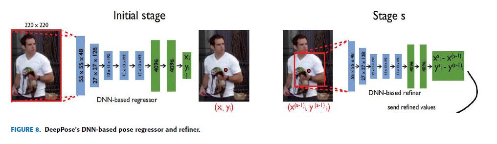
DeepPose has a total of 3-stages cascade of regressors to estimate the pose of an individual in a given image.
The Overall network structure of DeepPose is shown in Fig.8, in which the blue color shows the convolutional layers while the green shows the fully connected layers.
The left schematic view shows the initial stage which contains the DNN-based regressor for the coarse pose.
When joints are predicted at this stage, the image is cropped around the coordinates of the detected joint then passed to the next stage called the DNN-based refiner (on the right side of Fig.8) as an input.

DeepPose는 주어진 이미지에서 개인의 pose를 estimate하기 위해 총 3-stages cascade of regressors를 가지고 있다.
DeepPose의 전체 network 구조는 Fig.8에 나타나 있으며, 파란색은 convolutional layers를 나타내고 녹색은 fully connected layers를 보여준다.
왼쪽 개략도는 coarse(거친) pose에 대한 DNN-based regressor를 포함하는 초기 단계를 보여준다.
이 단계에서 joints가 예측되면 영상이 검출된 joint의 좌표 주변을 자른 다음 DNN 기반 정제기(그림 8의 오른쪽)라고 하는 다음 단계로 입력으로 전달됩니다.

The performance of this model is evaluated on two datasets (FLIC and LSP) using evaluation metrics of PCK and PCP.
This model outperformed the previous SOTA works in most cases.

이 모델의 성능은 PCK 및 PCP의 평가 지표를 사용하여 두 개의 datasets(FLIC, LSP)에서 평가된다.
이 모델은 대부분의 경우 이전 SOTA 작업보다 성능이 우수하다.

Even though producing the first CNN based human pose estimation model is very significant, the work has some limitations.
The main problem was regressing to a location is very difficult.
This increased the complexity of the learning which weakened generalization.
Thus, DeepPose performed very poorly in some regions.
However, it has been very helpful for recent SOTA researches to change the challenge to the problem of estimating heatmaps for available joints or keypoints.

first CNN based human pose estimation model을 생산하는 것은 매우 중요하지만, 이 작업은 몇 가지 한계를 가지고 있다.
가장 큰 문제는 location로 regressing하는 것이 매우 어렵다는 것이었다.
이것은 일반화를 약화시키는 학습의 복잡성을 증가시켰다.
따라서 DeepPose는 일부 regions에서 매우 낮은 성능을 보였다.
그러나 최근의 SOTA 연구에서 사용 가능한 joints 또는 keypoints에 대한 heatmaps 추정 문제로 문제를 변경하는 것은 매우 도움이 되었다.

B. ConvNet POSE: EFFICIENT OBJECT LOCALIZATION USING CONVOLUTIONAL NETWORKS

In this paper [70], ConvNet architecture, multi-resolution CNN architecture is proposed to generate discrete heatmaps instead of continuous regression that predicts the probability of the location of individual joints in monocular RGB images.
In ConvNet pose, different scale features are captured simultaneously using multiple resolution CNN architectures in parallel.

본 논문에서는 monocular RGB images에서 individual join의 위치 확률을 예측하는 continuous regression 대신 discrete heatmaps을 생성하기 위해 multi-resolution CNN architecture를 제안한다.
ConvNet 포즈에서는 multiple resolution CNN architectures를 병렬로 사용하여 different scale features이 동시에 캡처된다.

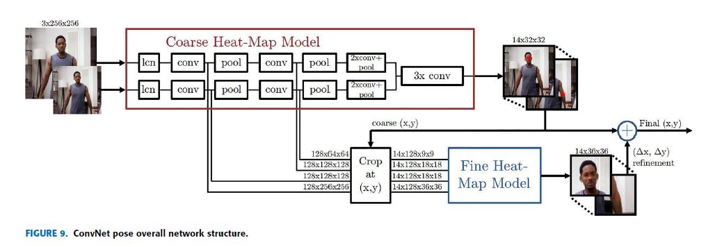
This model implements a sliding window detector that produces a coarse heatmap output and this coarse heatmap is refined by ‘pose refinement’ ConvNet to get better localization which improves in recovering the spatial accuracy lost due to pooling in the initial model.
This means the model contains a module (a convolutional network) for coarse localization, a module for sampling and cropping the features of ConvNet for each joint at a specified location (x, y), and also a module for fine-tuning as shown in Fig.9 which displays the model’s overall network structure.

이 모델은 coarse heatmap 출력을 생성하는 sliding window detector를 구현하고, 이 coarse heatmap는 initial model의 pooling으로 인해 손실된 공간 정확도를 recovering을 개선하는 더 나은 localization을 얻기 위해 ‘pose refinement’ ConvNet에 의해 정제된다.
이는 모델에

1. coarse localization을 위한 module(a convolutional network),
2. 지정된 location(x, y)에서 각 joint에 대한 ConvNet의 features를 sampling하고 cropping을 위한 module,
3. 그리고 모델의 전체 network 구조를 나타내는 그림 9에 표시된 것처럼 fine-tuning을 위한 module이
   포함되어 있다는 것을 의미한다.

This model has shown the use of a ConvNet and a graphical model jointly.
The spatial relationship between the joints is typically learned by the graphical model [71].
The performance of the model is evaluated using PCK and PCKh@0.5 on FLIC [61] and MPII [22] dataset respectively in which outperformed the previous SOTA models.

이 모델은 ConvNet과 graphical model을 jointly(공동)하게 사용하는 것을 보여주었다.
joints 사이의 공간 관계는 일반적으로 graphical model에 의해 학습된다[71].
모델의 성능은 각각 이전 SOTA 모델을 능가한 FLIC [61] 및 MPII [22] dataset에서 PCK 및 PCKh@0.5를 사용하여 평가된다.

This model implemented the joint use of a convolutional network and graphical model.
Also, it revealed heatmaps are preferable than direct joint regression.
Human poses are structured because of physical connections (like knees are rigidly related to hips and ankles), body part proportions, joint limits (like knees do not bend forward), left-right symmetries, interpenetration constraints, and others.
Thus, modeling this structure realizes that detecting visible keypoints is easier and this directs on estimating the occluded keypoints which are very hard to detect.
However, this model lacks structure modeling.

이 모델은 convolutional network와 graphical model의 공동 사용을 구현했다.
또한, heatmaps이 direct joint regression보다 더 바람직하다는 것을 밝혀냈습니다.
Human poses는 신체 연결(무릎은 발목과 엉덩이에 강하게 관련되는 것처럼), body part 비율, 관절 한계(무릎이 앞으로 구부러지지 않음), 좌-우 대칭, 삽입 제약 등으로 인해 구조화된다.
따라서, 이 구조를 모델링하는 것은 가시적인 keypoints를 detect하는 것이 더 쉽다는 것을 깨닫고 이것은 detect하기 매우 어려운 occluded(가려진) keypoints를 추정하는 데 도움이 된다.
그러나 이 모델에는 구조 모델링이 없다.

C. CPM: CONVOLUTIONAL POSE MACHINES

CPM [29] consists of a sequence of convolutional networks that produce a 2D belief map for the location of each keypoint.
The sequential prediction framework provided by CPM helps them to learn rich implicit spatial information and feature representation of images at the same time.
CPM is completely differentiable and the multi-stage architecture can be trained end-to-end.
Thus, the image features and belief maps produced by the previous stage are given as input for the next stage (except the first stage) in CPM.
One of the basic motivations for CPM is learning long-range spatial relationships and this is done using large receptive fields.
Also, CPM used intermediate supervision after each stage to avoid the problem of vanishing gradients.

CPM [29]은 각 키포인트 위치에 대한 2D 믿음 맵을 생성하는 일련의 컨볼루션 네트워크로 구성된다.
CPM이 제공하는 순차적 예측 프레임워크는 풍부한 암묵적 공간 정보와 이미지의 특징 표현을 동시에 학습하는 데 도움이 된다.
CPM은 완전히 차별화되며 다단계 아키텍처를 종단 간 훈련할 수 있다.
따라서 이전 단계에서 생성된 영상 특징과 신념 맵은 CPM의 다음 단계(1단계 제외)에 대한 입력으로 제공된다.
CPM의 기본 동기 중 하나는 장거리 공간 관계를 학습하는 것이며 이는 대규모 수용 필드를 사용하여 수행된다.
또한, CPM은 각 단계마다 중간 감독을 사용하여 구배 현상이 사라지는 문제를 피했다.

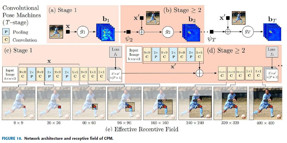
The overall network structure and receptive field of CPM are shown in Fig.10.
CPM network is divided into multiple stages (the stage is used as hyper-parameter, usually D3) and at each stage, the confidence (belief) map of each keypoint is computed. Fig.10, (a) and (b) show the structures in the pose machine, (c) and (d) show the corresponding convolutional networks respectively, while (e) shows the receptive fields at different stages.

전체적인 network 구조와 CPM의 receptive field는 그림 10과 같다.
CPM network는 multiple stages(stage가 hyper-parameter, 보통 D3으로 사용됨)로 나뉘며, 각 stage에서 각 keypoint의 confidence (belief) map을 계산한다.
Fig.10, (a) 및 (b)는 pose machine의 구조를 보여주고, (c)와 (d)는 각각 대응하는 convolutional networks를 보여주고, (e)는 다른 stages에서 receptive fields를 보여준다.

At the first stage a basic convolutional network, a classic VGG structure represented by X predicts the belief maps of each keypoint from the original input image.
This leads to the condition that if the individual in the image has p joint points, then the belief map has p layers with each layer representing the joint point heatmap.
Each layer’s loss is added up as a total loss to achieve intermediate supervision which helped them in vanishing gradients.

첫 번째 stage에서 기본 convolutional network, X로 나타내는 classic VGG 구조는 original input image에서 각 keypoint의 belief maps을 예측한다.
이것은 만약 영상의 개인이 p joint points을 가지고 있다면, belief map은 joint point heatmap을 나타내는 각 레이어를 가지고 있다는 조건으로 이어진다.
vanishing gradients문제를 돕는 intermediate supervision을 하기위해 각 layer의 loss는 total loss로 합산된다.

For subsequent stages, stage \(\ge 2\), the structure is the same except the input to the network are two data: a belief map output from the previous stage and the result of the original image passed through X’.
In addition to that, CPM showed that increasing the receptive field increases the accuracy of the prediction of keypoints.
Furthermore, CPM implemented intermediate supervision after each stage to solve the vanishing gradients.

후속 stages(stage \(\ge 2\))의 경우, 이전 단계의 belief map output과 X’를 통과하는 original image의 결과라는 두 가지 데이터가 network에서 input인것을 제외하면 구조는 동일하다.
또한, CPM은 수용 필드를 늘리면 keypoints 예측의 정확도가 높아진다는 것을 보여주었다.
또한, CPM은 각 stage마다 intermediate supervision을 실시하여 vanishing gradients 문제를 해결하였다.

CPM implemented their model on three known datasets: MPII, LSP, and FLIC using evaluation metrics of PCK@0.1, PCK@0.2, and PCKh@0.5.
It is noteworthy to mention that CPM achieved a PCKh@0.5 score of 10.76% higher than the previous SOTA on the most challenging part, the ankle.

CPM은 PCK@0.1, PCK@0.2, PCKh@0.5의 평가 지표를 사용하여 MPII, LSP, FLIC의 three known datasets에 모델을 구현했다.
가장 어려운 부분인 발목에서 CPM이 기존 SOTA보다 10.76%의 높은 PCKh@0.5 score을 달성했다는 점은 주목할 만하다.

CPM is the integration of the convolutional network to pose machines to learn image features and image-dependant spatial models to estimate human poses.
Nevertheless, this work implemented a top-down approach on single person pose estimation, which leads to known errors and complexities of the top-down approach discussed earlier.

CPM은 image features를 학습하기 위한 pose machines인 convolutional network와 human poses를 estimate하기 위한 image-dependant spatial models을 통합한 것이다. 그럼에도 불구하고, 이 연구는 single person pose estimation에 대해 top-down approach로 구현했고, 이는 앞에서 논의한 top-down approach의 알려진 errors와 복잡성으로 이어진다.

D. STACKED HOURGLASS NETWORKS FOR HUMAN POSE ESTIMATION

Stacked hourglass network [27], exactly lookalike of an hourglass stacked which are composed as steps of pooling and upsampling layers, is on the basic motivation of capturing information at every scale.
In human pose estimation: an individual’s orientation, limb arrangements, the relationship between adjacent joints, and other many cues that are best identified at different scales in a given image.

Stacked hourglass network[27]는 pooling 및 upsampling layers의 steps로 구성된 쌓여진 모래시계와 정확히 유사하며, 모든 scale의 정보를 캡처하는 기본 motivation에 있다.
human pose estimation에서: 개인의 방향, 사지 배열, 인접 관절 사이의 관계, 주어진 이미지에서 다른 scales로 가장 잘 식별되는 다른 많은 단서들.

Thus, the stacked hourglass network is performing a repeated use of bottom-up (from high resolution to low resolution using pooling), top-down (from low resolution to high resolution using upsampling), and intermediate supervision to improve the network performance.
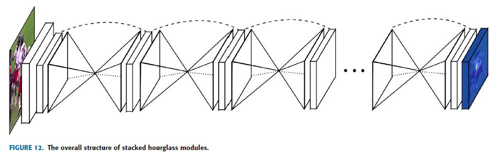
The overall network structure of stacked hourglass modules is given in Fig.12.
The hourglass stacked helps them to capture information on every scale means both global and local information is captured.
It means skip connections are used to preserve spatial information in every resolution and pass it for upsampling.

따라서 stacked hourglass network는 network 성능을 향상시키기 위해 bottom-up (pooling을 사용하여 high resolution부터 low resolution까지), top-down (upsampling을 사용하여 low resolution에서 high resolution까지), 그리고 intermediate supervision을 반복적으로 사용하여 수행하고 있다.
stacked hourglass modules의 전체적인 network 구조는 Fig.12에 제시되어 있다.
hourglass stacked은 그것들이 global과 local 정보가 모두 캡처된다는 것을 의미하는 모든 scale의 정보를 캡처하는 것을 돕는다..
즉, skip connections은 모든 resolution에서 공간 정보를 보존하고 그것을 upsampling해서 전달하기 위해 사용된다.

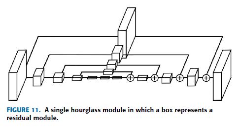
Fig.11 displays a single hourglass module in which a single box represents a residual module.
The primary module in an hourglass structure, residual or recurrent learning, is used for the bypass addition structure.
This residual learning, composed of three convolutional layers with different scales in which batch normalization and ReLu inserted between them, extracts higher-level features while maintaining the primary level of information.
The second path skips the path and contains only one kernel, A convolution layer with a scale of 1.
Thus, only the data depth is changed not the data size.

Fig.11은 single box가 residual module을 나타내는 single hourglass module을 보여준다.
hourglass 구조의 primary module인 residual 또는 recurrent learning은 bypass 추가 구조에 사용된다.
배치 정규화와 ReLu 사이에 삽입된 서로 다른 척도의 세 개의 컨볼루션 레이어로 구성된 이 잔류 학습은 기본 수준의 정보를 유지하면서 상위 수준의 특징을 추출한다.
두 번째 경로는 경로를 건너뛰고 하나의 커널, 즉 척도가 1인 컨볼루션 계층만 포함합니다.
따라서 데이터 크기만 변경되지 않고 데이터 깊이만 변경됩니다.

For each hourglass module, a fourth-order residual module is used.
The 4th-order Hourglass sub-network extracts features from the original scale to the 1/16 scale.
It does not change the data size, only the data depth.
The hourglass module is used to capture local information contained in pictures at different scales.
At different scales, it may contain a lot of useful information, such as the position of the human body, the movements of the limbs, the relationship between adjacent joint points, and so on.
First, the Conv layer and Max Pooling layer are used to scale features to a small resolution.
At each Max Pooling (down-sampling), the network forks (branches) and convolves the features with the original pre-pooled resolution;
After getting the lowest resolution features, the network starts up-sampling, and gradually combines feature information of different scales.
The lower resolution here uses the nearest neighbor upsampling method, and two different feature sets are added element by element (which performs two different feature sets Add elements).

각 hourglass module에 대해 4차 residual module이 사용된다.
4th-order Hourglass sub-network는 original scale에서 1/16 scale까지의 features을 추출한다.
data size는 변경되지 않고 data depth만 변경됩니다.
hourglass module은 사진에 포함된 local 정보를 다양한 scales로 캡처하는 데 사용됩니다.
다른 scales에서, 그것은 human body의 position, 팔다리의 움직임, 인접한 관절 points들 사이의 관계 등과 같은 많은 유용한 정보를 포함할 수 있다.
First, Conv layer와 Max Pooling layer는 scale features를 small resolution로 사용된다.
각 Max Pooling(down-sampling)에서 network는 original pre-pooled resolution로 features을 forks(branches)하고 convolves한다.
lowest resolution features을 얻은 후, network는 up-sampling을 시작하고 다양한 scales의 feature 정보를 점차 결합한다.
여기서 lower resolution는 nearest neighbor upsampling method을 사용하며, 요소별로 두 개의 다른 feature sets가 element by element로 추가됩니다(두 개의 다른 feature sets 추가 elements 수행).

In stacked hourglass down-sampling uses max pooling, and up-sampling uses nearest-neighbor interpolation.
The original image is down-sampled and input into the Hourglass sub-net.
The output of Hourglass goes through two linear modules to get the final response graph.
During this period, the Residual module and the convolutional layer are used to gradually extract features.
The secondary used network centered around two Hourglass and repeats the second (latter) half of the primary network.
The input of the second Hourglass contains three channels (paths): the input data of the first Hourglass, the output data of the first Hourglass, and the first-level prediction result.
These three channels of data are fused by concat and add, and their scales are different, which reflects the currently popular idea of skip-level (jump) structure.

stacked hourglass down-sampling에서는 max pooling을 사용하고 up-sampling에서는 nearest-neighbor interpolation을 사용한다.
original image은 down-sample되어 Hourglass sub-net에 입력된다.
Hourglass의 output은 두 개의 linear modules을 통해 final response graph를 얻는다.
이 기간 동안 Residual module과 convolutional layer가 점진적으로 features을 추출하는 데 사용된다.
secondary는 두 개의 Hourglass를 중심 network를 사용하고 primary network의 두 번째(나중에) half를 반복합니다.
second Hourglass의 input에는 다음 three channels (paths)를 포함한다 : 첫 번째 Hourglass의 input data, 첫 번째 Hourglass의 output data, first-level 예측 결과
이 data의 three channels은 concat과 add에 의해 융합되며, 그 scales은 서로 다르며, 이는 현재 널리 알려진 skip-level (jump) 구조의 개념을 반영한다.

In the Stacked hourglass network both high-resolution to low-resolution processing and low-resolution to high-resolution processing are symmetrical.
The stacked hourglass was tested on MPII and FLIC dataset benchmarks using PCK@0.2 and PCKh@0.5 evaluation metrics in which surpassed all previous SOTA performance.
In addition, this work has improved accuracy from 4-5%. on the joints difficult to detect (knees and ankles).

Stacked hourglass network에서는 high-resolution to low-resolution processing 과 low-resolution to high-resolution processing가 모두 대칭이다.
stacked hourglass는 이전의 모든 SOTA 성능을 능가하는 PCK@0.2 및 PCKh@0.5 평가 지표를 사용하여 MPII 및 FLIC ataset benchmarks에서 테스트되었다.
또한 이 작업은 감지하기 어려운 관절(골반과 발목)에 대해 정확도가 4-5%로 향상되었다.

E. DeeperCut: A DEEPER, STRONGER, AND FASTER MULTI-PERSON POSE ESTIMATION MODEL

DeeperCut [33] is a more similar and an upgrade version of the approach presented in DeepCut [52].
DeeperCut has implied a strong body part detectors to generate effective bottom-up proposals for body joints and adapted the extremely deep Residual Network (ResNet [38]) for human body detection whereas DeepCut adapted Fast R-CNN [48] for the task.
The proposed keypoints are assembled into a variable number of consistent body part configurations using image-conditioned pairwise terms.

DeepCut[33]은 DeepCut[52]에 제시된 approach의 업그레이드 버전이며 꽤 유사하다.
DeeperCut은 body joints에 대한 효과적인 bottom-up proposals을 생성하기 위해 strong body part detectors를 암시했으며 human body detection을 위해 deep Residual Network (ResNet)를 채택한 반면 DeepCut은 이 작업에 Fast R-CNN을 채택했다.
proposed keypoints는 image-conditioned pairwise terms를 사용하여 다양한 수의 일관된 body part configurations으로 조립된다.

Unlike DeepCut, DeeperCut used an incremental optimization strategy that explores the search space more efficiently which leads to both better performance and speed-up factors.
Adapting ResNet allowed this work to tackle the problem of vanishing gradients because ResNet tackles the problem bypassing the state though identity layers and modeling residual functions.

DeepCut과는 달리 DeeperCut은 search space를 보다 효율적으로 탐색하여 성능과 속도 향상 요인으로 이어지는 incremental optimization strategy을 사용했다.
ResNet을 적응시키면 ResNet은 identity layers를 통해 상태를 우회하는 문제를 해결하고 residual functions를 모델링하기 때문에 이 작업이 vanishing gradients 문제를 해결할 수 있었다.

Similar to DeepCut, DeeperCut jointly estimates the poses of every individual appeared in an image by minimizing a joint objective based on Integer Linear Programming (ILP).
The authors started by making a set of body joint candidates (D) generated by body part detectors and a set of body joint classes(C) such as head, shoulder, and knee in which each candidate’s joint has a unary score for every joint class.
Adapting ResNet to the fully convolutional model for the sliding window-based body part detection usually brings a stride of 32px which is too coarse for effective joint localization.
The authors showed by reducing the stride from 32px to 8px.
Besides, to tackling the problem of vanishing gradients in adapting ResNet, DeeeperCut also achieves a large receptive field size which allows them to incorporate context when predicting locations of individual body joints.

DeepCut과 마찬가지로 DeepCut은 Integer Linear Programming (ILP)에 기초한 공동 목표를 최소화하여 image에 나타난 모든 개인의 poses를 공동으로 estimates한다.
저자들은 body part detectors에서 생성된 a set of body joint candidates(D)와 joint class마다 unary score를 가지는 각 candidate의 joint인 머리, 어깨, 무릎 등 a set of body joint candidates(C)을 만드는 것으로 시작했다.
sliding window 기반 body part detection를 위해 ResNet을 fully convolutional model에 적용하는것은 효과적인 joint localization에는 너무 coarse한 a stride of 32px을 보통 가져온다.
저자들은 stride를 32px에서 8px로 줄임으로써 보여주었다.
또한, DeeeperCut은 ,ResNet 조정에서 vanishing gradients 문제를 해결하기 위해, 개인 body joints의 locations를 예측할 때 context를 통합할 수 있는 큰 receptive field size를 달성한다.

After detecting the keypoints, DeeperCut implemented image-conditioned pairwise terms on proposed keypoints.
First, an individual in the image is randomly selected and then the location is fixed for each keypoint at its ground truth location using the learned regression.
Second, an individual pairwise score-maps will be done and this gets the shape of a cone which extends to the direction of the correct location, but these are visually fuzzy.
Finally, by applying an incremental optimization strategy that uses a branch-and-cut algorithm to incrementally solve several pairwise instances to have a valid human pose configuration.

keypoints를 detecting한 후, DeepCut은 제안된 keypoints에 image-conditioned pairwise terms를 구현했다.
First, image의 individual을 임의로 선택한 다음 학습된 regression을 사용하여 ground truth location에서 각 keypoint에 대한 location을 고정한다.
Second, individual pairwise score-maps이 수행되고 이것은 correct location의 방향으로 확장되는 원뿔(cone) 모양을 얻지만, 이것들은 시각적으로 흐릿하다.
Finally, branch-and-cut algorithm을 사용하여 여러 pairwise의 instances를 점진적으로 해결하여 valid human pose configuration을 갖는 incremental optimization strategy을 적용함으로써.

DeeperCut employed the model on LSP, MPII, and COCO dataset using an evaluation metric of AP and mAP which outperformed most of the previous SOTA models except CPM [29] which got similar performance in some cases.
Evaluation is done on both single and multi-person pose estimation.

DeeperCut은 AP와 mAP의 evaluation metric를 사용하여 LSP, MPII, COCO dataset에 model을 사용했으며, 일부 경우 유사한 성능을 얻은 CPM[29]을 제외한 대부분의 이전 SOTA 모델을 능가했다.
평가는 single-person pose estimation와 multi-person pose estimation 모두에서 이루어진다.

DeeperCut has introduced novel image-conditioned pairwise terms but still needs several minutes per given image (around 4 min/image).
However, the pairwise representations are very hard to regress precisely.
Additionally, it implemented the model with a batch size of 1 which increases the instability of the model.

DeeperCut은 novel image-conditioned pairwise terms를 도입했지만 여전히 주어진 image당 몇 분(이미지 약 4분)이 필요하다.
그러나 pairwise representations은 정확하게 regress하기 어렵다.
또한 batch size가 1인 모델을 구현하여 모형의 불안정성을 높였다.

F. IEF: HUMAN POSE ESTIMATION WITH ITERATIVE ERROR FEEDBACK

IEF human pose estimation [72] basically motivated on the concept of prediction, identify what is wrong on this prediction, and correct them iteratively, which is done by a top-down feedback mechanism.
IEF employed a framework that extends the hierarchical feature extractor (ConvNet) to include both input and output spaces.
In IEF, Error predictions are fed to the initial solution repeatedly and progressively by a self-correcting model as a replacement of directly identifying the keypoints in one go.
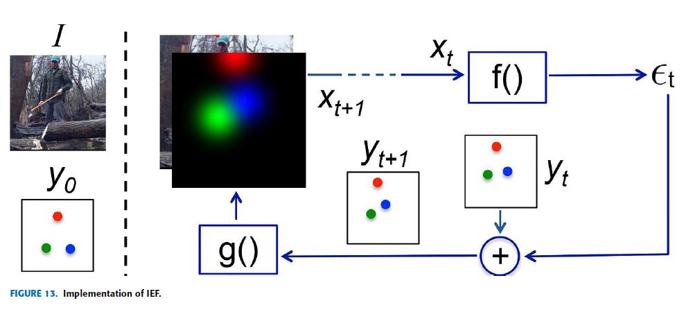
This framework is called Iterative Error Feedback (IEF) and Fig.13 shows the implementation of IEF for human pose estimation.

IEF human pose estimation은 기본적으로 예측의 개념에 동기를 부여하고, 이 예측에서 무엇이 잘못되었는지 식별하며, top-down feedback mechanism에 의해 수행되는 반복적 수정이다.
IEF는 input space와 output space를 모두 포함하도록 계층적 feature extractor(ConvNet)를 확장하는 framework를 채택했다.
IEF에서 오류 예측은 keypoints를 직접 한 번에 식별하는 대체물로 self-correcting model에 의해 반복적으로, 또 점진적으로 초기 솔루션에 공급된다.
이 framework는 반복 오류 피드백(IEF)이라고 하며 Fig.13은 human pose estimation을 위한 IEF의 구현을 보여준다.

On the left side of Fig.13, there is an input composed of the image I and the initially guessed keypoints \(y_0\) (representation of the previous output \(y_{t-1}\)).
Assume three keypoints to the head (red), the right wrist (green), and the left wrist (blue).
Then, define input \(X_t = I \oplus g(y_{t-1})\), where I represents the image and \(y_{t-1}\) is the previous output.
The function \(f(X_t)\), modeled as a ConvNet, produces the correction \(\varepsilon_t\) as output and this output is added to the current output \(y_t\) to produce \(y_{t+1}\) which means the correction is considered.
The function \(g(y_{t+1})\) converts every keypoint position into one Gaussian heatmap channel so that it can be part of the input with the image for the next iteration.
This procedure is done repeatedly and progressively T times until getting a refined \(y_{t+1}\) which is very close to the ground truth.

Fig.13의 왼쪽에는 image I와 초기에 추측된 keypoints \(y_0\)(이전 output \(y_{t-1}\)의 representation)로 구성된 input이 있다.
머리(빨간색), 오른쪽 손목(녹색), 왼쪽 손목(파란색)의 세 가지 keypoints를 가정한다.
그런 다음, input은 \(X_t = I \oplus g(y_{t-1})\) 로, \(y_{t-1}\)는 이전 output으로 정의한다. ConvNet으로 모델링된 function \(f(X_t)\)는 correction \(\varepsilon_t\)를 output으로 생성하며 이 output은 현재 output \(y_t\)에 추가되어 \(y_{t+1}\)을 생성하고 이것은 correction이 고려됨을 의미한다.
function \(g(y_{t+1})\)는 모든 keypoint position을 하나의 Gaussian heatmap channel로 변환하여 다음 iteration을 위한 image와 함께 input의 일부가 될 수 있도록 한다.
이 절차는 ground truth에 매우 가까운 정제된 \(y_{t+1}\)를 얻을 때까지 반복적이고 점진적으로 T번 수행된다.

IEF human pose estimation evaluated their performance on two datasets (LSP and MPII) using a single evaluation metric PCKh@0.5. IEF introduced novelty and good work.
The functions used, both \(f\) and \(g\), are learnable and also, \(f\) is a ConvNet.
This means \(f\) has the ability to learn features over the joint input-output space.

IEF human pose estimation은 single evaluation metric PCKh@0.5를 사용하여 두 datasets(LSP, MPII)에서 성능을 평가했다.
IEF는 novelty와 좋은 일을 소개했다.
사용된 함수 \(f\)와 \(g\) 모두 학습 가능하며 \(f\)는 ConvNet이다.
이는 \(f\)가 joint input-output space에 걸쳐 features을 학습할 수 있다는 것을 의미한다.

G. REALTIME MULTI-PERSON2D POSE ESTIMATION USING PART AFFINITY FIELDS

Realtime multi-person 2D pose estimation [34] proposed a novelty approach to connect human body parts using Part Affinity Fields (PAF), a non-parametric method, to achieve bottom-up multi-person pose estimation model.
The main motivation of this research is identifying the difficulties faced on detecting individual body joints involving multi-person such as the number of people in the image (infinity), the interaction between these people, irregular scale for each individual, increasing complexity, and others.

Realtime multi-person 2D pose estimation은 bottom-up multi-person pose estimation model을 달성하기 위해 non-parametric method인 Part Affinity Fields (PAF)를 사용하여 human body parts를 연결하는 novelty approach을 제안했다.
이 연구의 main motivation은 image 내 사람 수(무한정), 이들 사람 간의 interaction, 각 개인에 대한 불규칙한 scale, 복잡성 증가 등 multi-person이 포함되는 개별 body joints을 감지하는 데 직면하는 어려움을 식별하는 것이다.

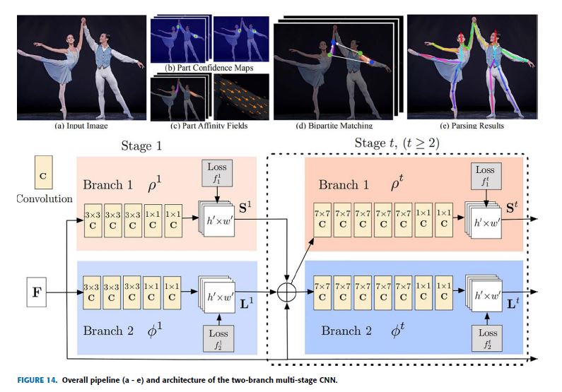
The overall pipeline and architecture of this model are shown in Fig.14.
For a given input image (Fig.14. a), the location of each joint is determined by part confidence maps (Fig.14. b), and the location and orientation of the body parts are determined by PAF (Fig.14. c) a 2D vector that represents the degree of association between the body parts.
These body part candidates are associated with the parsing step to perform a set of bipartite matching as shown in Fig.14 (d) and finally, assembled full-body pose because of parsing results in (e).

이 모델의 전체적인 pipeline과 구조는 Fig.14에 나타나 있다.
주어진 input image (Fig.14. a)의 경우, 각 joint의 location은 part confidence maps (Fig.14. b)에 의해 결정되며, body parts의 location와 orientation은 body parts 사이의 연관 정도를 represent하는 2D vector인 PAF (Fig.14. c)에 의해 결정된다.
이러한 body par 후보들은 Fig.14 (d)에 표시된 대로 일련의 초당적 일치를 수행하기 위한 구문 분석 단계와 연관되어 있으며 마지막으로 (e)의 구문 분석 결과 때문에 full-body pose를 취합했다.

The two-branch multi-stage CNN network shown in Fig.14 receives an input of a feature map F of an image initialized by the first 10 layers of VGG architecture.
The feed-forward model simultaneously predicts confidence maps S (shown in beige) for predicting the location of joints with J confidence maps for each joint \((S = S_1, S_2, . . . , S_J)\) and affinity fields L or a set of 2D vector fields (shown in blue) for encoding parts/limbs association which has C vectors corresponding to each limb \((L = L_1, L_2, . . . , L_C)\).

Fig.14에 표시된 two-branch multi-stage CNN network는 VGG architecture의 처음 10 layers에 의해 초기화된 이미지의 feature map F의 input을 받는다.
feed-forward model은 각 joint \((S = S_1, S_2, . . . , S_J)\)에 대한 “J confidence maps” 및 “affinity fields L” 또는 각 limb \((L = L_1, L_2, . . . , L_C)\)에 해당하는 C vectors를 가지는 parts/limbs association를 encoding 하기위한 “a set of 2D vector fields” (shown in blue)를 사용하여 joints의 location을 예측하기 위한 confidence maps S (shown in beige)를 동시에 예측한다.

Thus, at the end of the first stage, the network outputs a set of detection confidence maps and part affinity fields.
For the consecutive stages, the inputs will be the combination of the two previous stage outputs and the feature map F.
Both the confidence maps and the part affinity fields are passed by the greedy inference to have the 2D keypoints for every individual in the image, called Bipartite matching.
Furthermore, this work implemented intermediate supervision after each stage to solve the vanishing gradient’s problems by restoring the gradients periodically.

따라서, first stage가 끝날 때, network는 a set of detection confidence maps과 part affinity fields를 outputs다.
consecutive stages의 경우, inputs은 두 이전 stage outputs과 feature map F의 조합이 된다.
confidence maps과 part affinity fields 모두 image 내의 모든 개인에 대한 2D keypoints를 가지기 위한 Bipartite matching라고 부르는 탐욕 추론을 통과한다.
또한, 이 작업은 각 stage 후에 intermediate supervision을 구현하여 주기적으로 gradients를 복원하여 vanishing gradient 문제를 해결했다.

This work is evaluated on COCO and MPII dataset using AP, mAP, and PCKh@0.5 evaluation metrics to achieve the best results compared to the existing SOTA models in terms of performance and efficiency.

본 연구는 성능 및 효율성 측면에서 기존 SOTA 모델과 비교하여 최상의 결과를 얻기 위해 AP, mAP 및 PCKh@0.5 평가 지표를 사용하여 COCO 및 MPII 데이터 세트에서 평가된다.

H. CPN: CASCADED PYRAMID NETWORK FOR MULTI-PERSON POSE ESTIMATION

Cascaded Pyramid Network (CPN) for multi-person pose estimation model [32] is motivated with the concept of facing the challenging problems which are called “hard keypoints”.
These include occlusion of keypoints (Occluded by clothes or another person), invisible keypoints, complex backgrounds, etc.
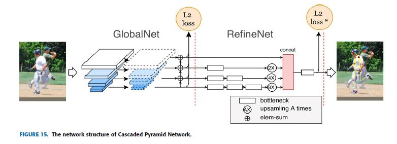
The authors proposed a top-down model for multi-person pose estimation with CPN network structure as shown in Fig.15.
This CPN network structure is composed of two stages: GlobalNet and RefineNet.
Relatively easy keypoints are estimated by the GlobalNet while the hard keypoints estimation is done by RefineNet using online hard keypoint mining loss.

multi-person pose estimation model을 위한 계단식 피라미드 네트워크(CPN)는 “hard keypoints”라고 불리는 어려운 문제에 직면한다는 개념에 동기 부여가 되었다.
여기에는 keypoints의 occlusion(옷이나 다른 사람이 포함), invisible keypoints, 복잡한 배경 등이 포함된다.
저자들은 Fig.15와 같이 CPN network 구조를 가진 multi-person pose estimation을 위한 top-down model을 제안했다.
이 CPN network 구조는 다음 두 단계로 구성된다 : GlobalNet 및 ClearateNet.
비교적 easy keypoints는 GlobalNet에 의해 추정되고, hard keypoints 추정은 online hard keypoint mining loss을 사용하여 RefineNet에 의해 이루어진다.

CPN network structure uses a CNN model to identify some human keypoints called Visible easy keypoints, which are relatively easy to detect; for instance Nose, Left elbow, and right hand in the image below.
Visible easy keypoints have somewhat a fixed shape and this helps in obtaining texture information which makes it easy to get contextual information around the location of the joints.
Then there are visible hard keypoints that are obscured by clothes such as the left knee, right knee, and left hip.
Additionally, some joints are hidden and hard to distinguish, not only obscured by clothes, such as the right shoulder in the image shown below.
For such hard keypoints, which have no contextual information, increasing the local receptive field is required such that the context information can be further refined.
Based on this concept CPN roughly categorized the human body joints into simple parts and difficult parts.

CPN network 구조는 CNN model을 사용하여 상대적으로 쉽게 detect할 수 있는 Visible easy keypoints라고 하는 일부 human keypoints를 식별하는데, 예를 들어 아래 이미지에서 코, 왼쪽 팔꿈치 및 오른손을 사용한다.
눈에 보이는 쉬운 키포인트는 어느 정도 fixed shape를 가지고 있으며, 이는 관절의 위치 주변에서 상황 정보(contextual information)를 쉽게 얻을 수 있도록 하는 texture information를 얻는 데 도움이 된다.
그런 다음 왼쪽 무릎, 오른쪽 무릎, 왼쪽 엉덩이 등 옷에 가려 보이는 visible hard keypoints가 있다.
또한 일부 joints은 아래 보이는 것과 같이 image의 오른쪽 어깨와 같이 옷으로 가려져 구별하기 어렵다.
contextual information이 없는 이러한 hard keypoints의 경우 context information을 더욱 세분화할 수 있도록 local receptive field를 늘려야 한다.
이 개념을 바탕으로 CPN은 human body joints을 simple parts와 difficult parts으로 대략 분류했다.

GlobalNet, composed of a forward CNN, is a simple regression model that focuses on easy to detect human keypoints usually eyes, arms, and other easy to detect parts.
The purpose of RefineNet is to detect difficult-to-recognize human keypoints, called hard keypoints.
RefineNet integrates multiple receptive fields information with the feature maps of the pyramid model generated by GlobalNet.
Then finally all feature maps with the same size are concatenated such that a correction for ambiguous keypoints is obtained.
RefineNet applies two things to mine the difficult keypoints 1) concat when using features of multiple layers and 2) online hard keypoints mining technology for the second-level network.
In general, RefineNet combines low-level features and high-level features through convolution operations.

forward CNN으로 구성된 GlobalNet은 보통 눈, 팔 및 기타 detect하기 쉬운 human keypoints을 detect하는 데 초점을 맞춘 simple regression model이다.
RefineNet의 목적은 hard keypoints라고 불리는 difficult-to-recognize human keypoints를 감지하는 것이다.
RefineNet은 GlobalNet에서 생성한 pyramid model의 feature maps과 multiple receptive fields information를 통합한다.
그런 다음 마지막으로 same size인 all feature maps을 연결하여 애매한 keypoints를 보정한다.
RefineNet은 difficult keypoints를 mine하기 위해 2가지를 적용한다 : 1) multiple layers의 features을 사용할 때 concat, 2) second-level network를 위한 online hard keypoints mining technology
일반적으로, RefineNet은 convolution 작업을 통해 low-level features와 high-level features을 결합한다.

By the use of RefineNet plus online hard keypoints mining, the model outperformed the previous SOTA models when implementing the model on the COCO dataset using AP and OKS evaluation metrics.
CPN exhibits similar properties as stacked hourglass being symmetrical in both processing of high-to-low resolution and low-to-high resolution.
It is easy to observe processing from high-resolution to low-resolution as part of a classification network and that it is heavy.
Nevertheless, other-way processing (low-resolution to high Resolution) is relatively light.

RefineNet과 online hard keypoints mining을 사용하여, 모델은 AP 및 OKS 평가 지표를 사용하여 COCO dataset에 모델을 구현할 때 이전 SOTA 모델을 능가했다.
CPN은 high-to-low resolution 및 low-to-high resolution 모두 처리에서 대칭(symmetrical)을 이루는 stacked hourglass와 유사한 특성을 보인다.
classification network의 일부로 high-resolution부터 low-resolution까지의 processing를 관찰하기 쉽고 heavy하다.
그럼에도 불구하고 other-way processing (low-resolution to high Resolution)는 상대적으로 light하다.

I. SIMPLE BASELINES FOR HUMAN POSE ESTIMATION AND TRACKING

The main motivation behind simple baselines for human pose estimation and tracking [31] is that most of the recent models on human pose estimation are very complex and look different in structure but achieving very close results.
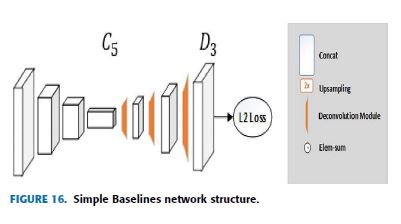
simple baselines proposed a relatively simplified and intuitive model that consists of a few deconvolutional layers at the end of ResNet to estimate the keypoints heatmap.
While most human pose estimation models like stacked hourglass [27] and CPN [32] use the structure composed of upsampling and convolution to increase the low-resolution feature map, simple baselines inserts several layers of deconvolution in ResNet which is a very simple way to expand the feature map to the size of the original image to generate the keypoints heatmap as shown in Fig.16.

human pose estimation 및 tracking을 위한 simple baselines의 main motivation은 human pose estimation에 대한 대부분의 최신 모델이 매우 복잡하고 구조적으로 다르게 보이지만 매우 가까운 결과를 달성한다는 것이다.
simple baselines은 keypoints heatmap을 추정하기 위해 ResNet 끝의 몇 개의 deconvolutional layers로 구성된 비교적 단순하고 직관적인 모델을 제안했다.
stacked hourglass와 CPN과 같은 대부분의 human pose estimation models은 low-resolution feature map을 증가시키기 위해 upsampling과 convolution으로 구성된 구조를 사용하지만, simple baselines은 ResNet에 여러 layers의 deconvolution을 삽입하는데, keypoints heatmap을 생성하기 위해 feature map을 original image 크기로 확장하여는 매우 간단한 방법이다. Fig.16에서 보듯이

In this article, both pose estimation and pose tracking are discussed, but our discussion focused on the former. As mentioned earlier this model’s network structure is straightforward: add several layers of deconvolution after ResNet to generate a heatmap for the individual keypoints.
The takeaway from this work is that the more the deconvolution layers, the greater the resolution of the generated heatmap.

이 논문에서, pose estimation과 pose tracking 모두에 대해 모두 논의하지만, 우리의 논의는 전자에 초점을 맞췄다. 앞에서 언급했듯이 이 모델의 network 구조는 간단하다: ResNet 이후 deconvolution layers를 여러 개 추가하여 개인 keypoints에 대한 heatmap을 생성한다.
이 작업의 단점은 deconvolution layers가 많을수록 생성된 heatmap의 resolution이 크다는 것이다.

Simple baselines achieved better performance compared to the previous works with the COCO dataset using AP evaluation metrics simply and easily.
Similar to CPN, high-resolution to low-resolution processing is viewed as part of a classification network (such as ResNet and VGGNet), and this is heavy while processing low-resolution to high-resolution is comparatively light.

Simple baselines은 단순하고 쉽게 AP 평가 지표를 사용하여 COCO dataset를 사용한 이전 작업에 비해 더 나은 성능을 달성했다.
CPN과 유사하게, high-resolution에서 low-resolution processing은 (ResNet와 VGGNet 같은)classification network의 part로 간주되며, 이는 무거운 반면 low-resolution에서 high-resolution processing은 상대적으로 가볍다.

J. HRNet: DEEP HIGH-RESOLUTION REPRESENTATION LEARNING FOR HUMAN POSE ESTIMATION

The usual trend applied in human pose estimation is downsampling high-resolution feature maps to low-resolution and then trying to recover a high-resolution value from low-resolution feature maps.
Based on this motivation, this research proposed an intuitive and different model called High-Resolution Net (HRNet) to maintain a high-resolution representation throughout the process [35].
In Stacked hourglass [27] both high-to-low resolution and low-to-high resolution processes are symmetrical.
Processing from high-resolution to low-resolution in both CPN [32] and simple baselines [31] considered as part of a classification network by the backbone architecture which is heavy, but the reverse process is relatively light.

human pose estimation에 적용되는 일반적인 trend는 high-resolution feature maps을 low-resolution feature maps으로 downsampling한 다음 low-resolution feature maps에서 high-resolution value을 복구하려고 시도하는 것이다.
이러한 motivation을 바탕으로, 본 연구는 process 전반에 걸쳐 high-resolution representation을 유지하기 위해 High-Resolution Net(HRNet)로 불리는 직관적이고 차별되는 model을 제안했다.
Stacked hourglass에서 high-to-low resolution 와 low-to-high resolution processes 모두는 대칭이다.
CPN과 simple baselines 모두에서 high-resolution부터 low-resolution까지의 Processing은 무거운 backbone 아키텍처에 의해 classification network의 part로 간주되지만, reverse process는 비교적 가볍다.

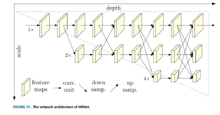
There is a high-resolution sub-network at the first stage of this network architecture, as shown in Fig.17.
Then gradually a high-to-low resolution sub-networks are added one by one to acquire the output of multiple stages.
Finally, the output of multiple resolution sub-networks in parallel are connected.
It performs repeated multi-scale fusions such that each high-resolution to low-resolution feature map representation can receive information from other parallel representation branches, again and again, to obtain a more informative high-resolution representation.
In the end, the keypoints heatmap of the network output and the spatial resolution are more accurate.
Because of repeated multi-scale fusions, HRNet does not need to use intermediate heatmap supervision, unlike the previous works.

Fig.17과 같이 이 network 아키텍처의 first stage에는 high-resolution sub-network가 있다.
그런 다음 gradually하게 high-to-low resolution sub-networks가 하나씩 추가되어 multiple stages의 output을 얻는다.
마지막으로, multiple resolution sub-networks의 output이 병렬로 연결된다.
그것은 high-resolution to low-resolution feature map representation 각각이 다른 parallel representation branches에서 정보를 수신하여 보다 유익한 high-resolution representation을 얻을 수 있도록 반복된 multi-scale fusions을 수행한다. 결국, network output의 keypoints heatmap과 spatial resolution가 더 정확하다.
반복된 multi-scale fusions 때문에 HRNet은 이전 작업과 달리 intermediate heatmap supervision을 사용할 필요가 없다.

HRNet consists of parallel high-to-low resolution subnetworks with repeated information exchange across multi-resolution sub-networks (multi-scale fusion).
The horizontal and vertical directions correspond to the depth of the network and the scale of the feature maps, respectively.
There are three scale branches in total.
The resolution of the feature map will not change during the forward propagation of each scale branch.
Even though there will be information exchange between each scale branch, the three branches are different.
For instance, in the forward process, branch 1 (the top branch in the figure) will downsample its feature map and then transfer it to branch 2.
Branch 2 will also send the enlarged feature to branch 1 through upsampling.
Two operations can be performed in the same stage.

HRNet은 multi-resolution sub-networks (multi-scale fusion)를 통한 반복적인 정보 교환이 있는 parallel high-to-low resolution subnetworks로 구성된다.
수평 방향과 수직 방향은 각각 network의 depth와 feature maps의 scale에 해당한다.
총 3개의 scale branches가 있다.
각 scale branch의 forward propagation 중에는 feature map의 resolution이 변경되지 않는다.
각 scale branch마다 정보 교환이 이루어지겠지만, three branches는 다르다.
예를 들어, forward process에서, branch 1 (the top branch in the figure)은 그것의 feature map을 downsample하고 그것을 branch 2로 전환할 것이다. Branch 2는 또한 확대된 feature을 upsampling을 통해 branch 1로 보낸다.
동일한 stage에서 두 가지 작업을 수행할 수 있다.

HRNet is evaluated on COCO and MPII dataset using AP, mAP, PCKh@0.5 evaluation metrics to achieve better performance.
HRNet introduced the connection of the outputs of high-to-low resolution sub-networks in parallel rather than the usual serial connection.
This means it does not require to restore the resolution because high-resolution representations are maintained always.

HRNet은 더 나은 성능을 달성하기 위해 AP, mAP, PCKh@0.5 평가 지표를 사용하여 COCO 및 MPII dataset에서 평가된다.
HRNet은 일반적인 직렬 연결이 아닌 병렬로 high-to-low resolution sub-networks의 outputs 연결을 도입했다.
즉, high-resolution representations이 항상 유지되므로 resolution을 복원할 필요가 없다.

K. CFA: CASCADE FEATURE AGGREGATION FOR HUMAN POSE ESTIMATION

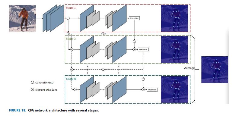
CFA proposed a cascaded multiple hourglass and aggregates low, medium, and high-level features to better capture local detailed information and global semantic information [26].
The motivation behind CFA network architecture is combining the concept implied in the network architecture of Stacked hourglass [27], CPN [32], and HRNet [35].

CFA는 cascaded multiple hourglass를 제안하고 local detailed information와 global semantic information을 더 잘 capture하기 위해서 low, medium, high-level features을 통합한다.
CFA network 아키텍처의 motivation은 Stacked hourglass, CPN, HRNet의 network 아키텍처에 내포된 개념을 결합하는 것이다.

The overall network structure of CFA is displayed in Fig.18.
CFA consists of multiple hourglass networks that are summed up by elements.
Feature aggregation shows that the hourglass network at each stage will predict the feature map, and the output of the previous layer is used as an input to the next stage at the same time.

CFA의 전체 network구조는 Fig.18에 표시되어 있다.
CFA는 elements로 요약되는 multiple hourglass networks로 구성된다.
Feature aggregation은 각 stage의 hourglass network가 feature map을 예측한다는 것을 보여주며, 이전 layer의 output이 다음 단계의 input으로 동시에 사용된다.

In each stage of CFA, ResNet based hourglass network is applied, which is an encoder-decoder model designed based on the hourglass.
The basic structure used for the encoder part is ResNet and the connection employed from the encoder to the decoder is highway connection.
There are three different feature aggregations in all stages of the CFA model: Low-level feature aggregation, middle-level feature aggregation, and high-level feature aggregation.

CFA의 각 stage에서, ResNet 기반 hourglass network가 적용되며, 이것은 hourglass를 기반으로 설계된 encoder-decoder model이다.
encoder 부분에 사용되는 기본 구조는 ResNet이고 encoder에서 decoder로 연결되는 연결은 highway connection이다.
CFA 모델의 모든 stages에는 Low-level feature aggregation, middle-level feature aggregation, high-level feature aggregation라는 세 가지 다른 feature 집계가 있습니다.

Fig.19 briefly describes the feature aggregation between different stages of CFA.
Detailed local information is accommodated in low-level features which help them in localizing the exact location of human joints.
On the other side, to refine the localization in case of complex backgrounds and partial occlusions, there are high-level features that contain semantic information.
Finally, all these different feature aggregations are forwarded as input for the next stage which brings prediction more stable.

Fig.19는 CFA의 서로 다른 stages 사이의 feature aggregation를 간략하게 설명한다.
Detailed local information은 human joints의 정확한 location을 localizing하는 데 도움이 되는 low-level features에 수용된다.
한편, 복잡한 배경과 부분적 occlusions의 경우 localization을 개선하기 위해, 의미 정보를 포함하는 high-level features이 있다.
마지막으로, 이러한 모든 다른 feature 집계는 예측을 보다 안정적으로 하는 다음 stage를 위한 input으로 전달된다.

CFA evaluated their model on the LIP and MPII datasets using only PCKh@0.5 evaluation metrics.
This paper is currently at the top of the 2019 CVPR article based on the MPII dataset PCKh@0.5 evaluation index in the field of single person pose estimation.

CFA는 PCKh@0.5 평가 지표만 사용하여 LIP 및 MPII datasets에서 모델을 평가했다.
본 논문은 현재 single person pose estimation에서 MPII dataset PCKh@0.5 평가 지수를 기반으로 한 2019년 CVPR 논문의 상위권에 있다.

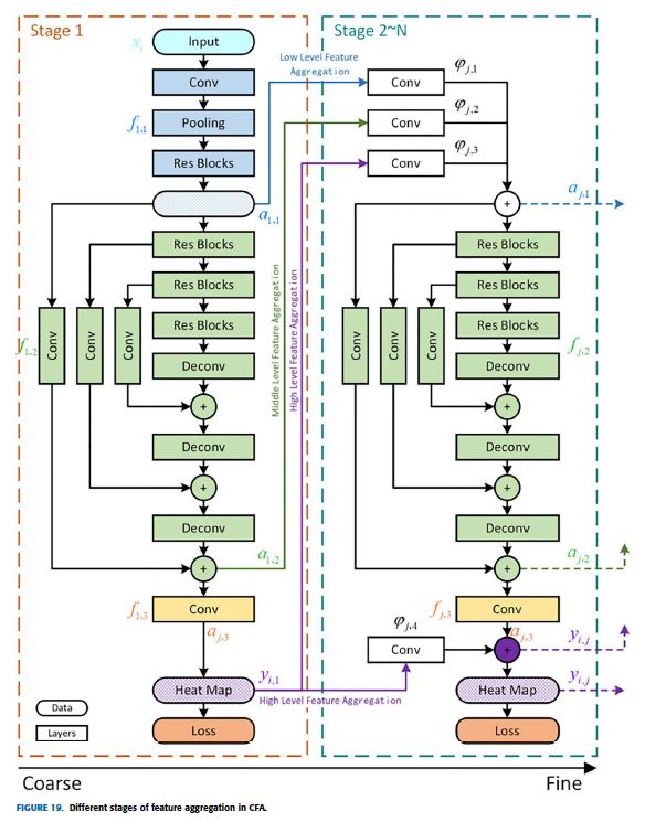
L. OccNet: HUMAN POSE ESTIMATION FOR REAL-WORLD CROWDED SCENARIOS

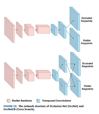
This model proposed in the motivation of estimating the pose of individuals in real-world crowded areas [73].
The challenges of estimating poses in such densely populated areas include people close to each other, mutual occlusions, and partial visibility.
The method is a two-stage, top-down approach that localizes the individual first and then performs a single-person pose estimation for every detected person.
This model proposed two occlusion detection networks Occlusion Net (OccNet) and Occlusion Net Cross Branch (OccNetCB) as shown in Fig.20,
the backbone network is ResNet shown in beige.

이 모델은 실제 밀집 지역에서 개인의 pose를 추정하는 motivation에서 제안되었다.
이러한 인구 밀집 지역에서 poses를 추정하는 challenges에는 서로 가까운 사람, mutual occlusions, partial visibility가 포함된다.
이 방법은 two-stage, top-down approach으로, 먼저 개인을 localize한 다음 detect된 모든 사람에 대해 single-person pose estimation을 수행한다.
이 모델은 Fig.20과 같이 두 개의 occlusion detection networks Occlusion Net(OccNet)과 Occlusion Net Cross Branch (OccNetCB)를 제안했다.
backbone network는 베이지색으로 표시된 ResNet이다.

In OccNet, to learn a joint representation in the previous layers the network splits after two transposed convolutions.
OccNet produces two sets of heatmaps for the location of keypoints per pose: a heatmap for visible keypoints and a heatmap for occluded keypoints.
The other architecture, OccNetCB, splits after only one transposed convolution.
In OccNetCB, both branches have the opportunity to get information extracted by one another because in OccNetCB the output from both layers is shared.

OccNet에서 이전 layers에서 joint representation을 학습하기 위해 두 개의 transposed convolutions 후 network가 분할된다.
OccNet은 pose당 keypoints의 location를 위한 두 세트의 heatmaps을 생성한다: 즉, visible keypoints를 위한 heatmap과 occluded keypoints를 위한 heatmap
다른 아키텍처인 OccNetCB는 단 하나의 transposed convolution 후에 분할된다.
OccNetCB에서는 OccNetCB에서 layers 모두에서 output이 공유되기 때문에 두 branches는 서로 추출한 정보를 얻을 수 있다.

The model has been evaluated on two datasets annotated on the crowded real-world situation: CrowdPose and JTA datasets using OKS and AP evaluation metrics.

모델은 혼잡한 실제 상황에 대해 라벨을 단 두 개의 datasets에서 평가되었다: OKS 및 AP 평가 지표를 사용하는 CrowdPose 및 JTA datasets.

M. DarkPose: DISTRIBUTION-AWARE COORDINATE REPRESENTATION FOR HUMAN POSE ESTIMATION

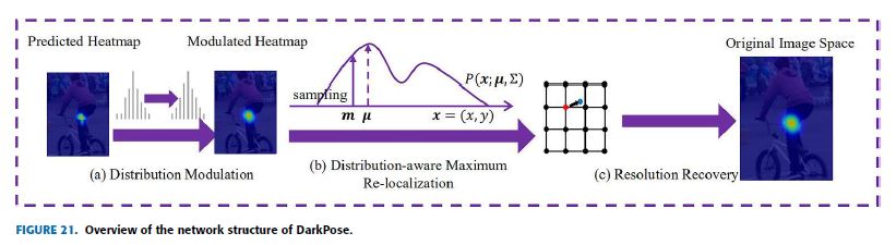
The main motivation behind the Distribution-Aware Coordinate Representation of Keypoint (DarkPose) is that the coordinate representation of the heatmap [30].
The assumption is that heatmap is never systematically investigated.
Based on this concept, the authors have shown design limitations on the existing standard coordinate decoding method, and propose a principled distribution-aware decoding method.
In addition to that, an accurate heatmap distribution for the unbiased model training instead of the usual coordinate encoding process is generated (i.e. transforming ground-truth coordinates to heatmaps).

Keypoint의 Distribution-Aware Coordinate Representation(DarkPose)의 main motivation는 heatmap의 좌표 표현이다.
heatmap은 결코 체계적으로 조사되지 않는다는 가정이다.
이 개념을 바탕으로 저자들은 기존 표준 좌표 디코딩 방법에 대한 설계 한계를 보여주었으며, 원칙적인 분포 인식 디코딩 방법을 제안한다.
또한 일반적인 좌표 인코딩 프로세스 대신 unbiased model training을 위한 정확한 heatmap 분포가 생성된다(즉, ground-truth 좌표를 heatmaps으로 변환).

Standard label representation in existing methods is coordinate heatmap as a 2-dimensional Gaussian distribution centered at the labeled coordinate of each keypoint of an individual.
According to this work, the major obstacle in heatmap label representation and that is quadratic function’s computational cost of the input image resolution which restrains CNN based models from processing the typically high-resolution raw imagery data.
Hence, there is a need to down-sample all the person bounding box images into a small resolution then fed them to human pose estimation model to predict the location of each keypoint in the original image coordinate space which needs to transform to the original coordinate space, and this brings the problem of sub-pixel localization.
Coordinate decoding from heatmap to coordinate is the last prediction of the location with the maximal activation.
The network structure of DarkPose is shown in Fig.21.

기존 methods의 표준 레이블 표현은 개인의 각 keypoint의 레이블링된 좌표를 중심으로 한 2차원 Gaussian distribution으로서 heatmap 좌표이다.
본 연구에 따르면, heatmap 레이블 표현의 주요 장애물이며, 이는 input image resolution에 대한 2차 함수(= quadratic function, MSE, L2 loss)의 계산 비용이며, 이는 CNN 기반 models가 일반적으로 high-resolution raw imagery data를 processing하지 못하도록 제한한다.
따라서 모든 person bounding box images를 small resolution로 down-sample한 다음 original 좌표 공간으로 변환해야 하는 original image 좌표 공간에서 각 keypoint의 location을 예측하기 위해 human pose estimation model에 공급해야 하며, 이로 인해 sub-pixel localization 문제가 발생한다.
heatmap에서 좌표까지의 좌표 decoding은 최대 활성화로 location의 마지막 예측이다.
DarkPose의 network 구조는 Fig.21에 나와 있다.

Coordinate representation, the problem of coordinate encoding and decoding, focused on predicting joint coordinates in a given image.
Coordinate decoding is a process of translating a predicted heatmap of each individual’s joint into a coordinate in the original image space.
Unlike the standard method of considering the second maximum activation to upsample the heatmaps to the original image resolution, DarkPose introduced the heatmap distributional statistics for disclosing the underlying maximum more accurately as shown in Fig.21 and this is employed using Taylor-expansion way.

좌표 encoding 및 decoding 문제인 좌표 표현은 given image에서 joint 좌표를 예측하는 데 초점을 맞췄다.
좌표 decoding은 각 개인의 joint의 예측 heatmap를 original image space에서 좌표로 translating하는 과정이다.
heatmap을 original image resolution로 upsample하기 위해 두 번째 maximum activation을 고려하는 표준 방법과 달리, DarkPose는 Fig.21과 같이 underlying maximum을 더 정확하게 공개하기 위한 heatmap distributional statistics를 도입했으며 이는 Taylor-expansion 방식을 사용하여 사용된다.

The heatmaps, predicted by a human pose estimation model, usually present multiple peaks around the maximum activation which causes negative effects on the performance of the decoding method.
To overcome this issue, DarkPose inserted modulating the heatmap distribution before resolution recovery.
In coordinate decoding method, three steps employed: heatmap distribution modulation, distributionaware joint localization by Taylor-expansion as sub-pixel accuracy, and resolution recovery to the original coordinate space.
A limitation similar to coordinate decoding is also observed in coordinate encoding in reducing the resolution.
Some of the existing methods start by downsampling given the original image to the model input size.
Therefore, in this case, transforming the ground-truth joint coordinates accordingly was necessary before generating heatmaps and this is done by using unbiased sub-pixel centered coordinate encoding.

human pose estimation model에 의해 예측된 heatmaps은 일반적으로 decoding method의 성능에 부정적인 영향을 주는 maximum activation 주위에 multiple peaks를 나타낸다.
이 문제를 극복하기 위해, DarkPose는 resolution recovery 전에 heatmap distribution를 modulating하는 것을 삽입했다.
좌표 decoding method에서는 3개의 steps가 이용된다 : heatmap distribution modulation, sub-pixel accuracy로 Taylor-expansion에 의한 distributionaware joint localization, original 좌표 공간에 대한 resolution recovery
resolution 감소의 coordinate encoding에서도 coordinate decoding과 유사한 limitation이 관찰된다.
기존 방법의 일부는 original image를 model input size에 맞게 downsampling하는 것으로 시작한다.
따라서, 이 경우 heatmaps을 생성하기 전에 그에 따라 ground-truth joint coordinates를 변환하는 것이 필요했으며, 이는 unbiased sub-pixel centered coordinate encoding을 사용하여 수행된다.

DarkPose has come up with the concept of problems facing in coordinate representation and the model was evaluated on COCO and MPII using evaluation metrics of PCK and OKS.

DarkPose는 좌표 표현에서 직면하는 문제의 개념을 고안했으며 모델은 PCK와 OKS의 평가 지표를 사용하여 COCO와 MPII에서 평가되었다.

V. SUMMARY AND DISCUSSION

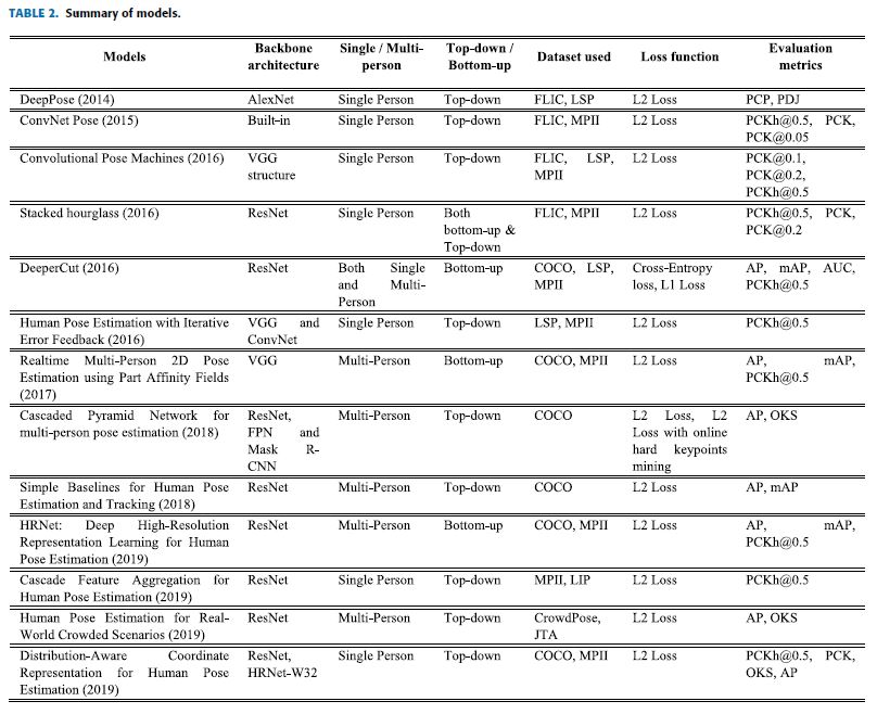
This paper reviewed the progress made in pose estimations for human beings with selected and most notable researches made to our knowledge.
This discussion started from Deep-Pose [46], the first well known and has been as reference for most researches in pose estimation progress.
Then models have been selected based on their novelty, innovation, the influence made by the model, and other criteria.
Table 2 summarizes the models with some criteria.

본 논문은 우리의 지식에 대해 수행된 선별적이고 가장 주목할 만한 연구를 통해 인간에 대한 pose estimations에서 이루어진 진행 상황을 검토했다.
이 논의는 처음 잘 알려진 Deep-Pose에서 시작되었으며 pose estimation progress에서 대부분의 연구에 reference로 사용되어 왔다.
그 후 모델은 새로움, 혁신, 모델에 의해 만들어진 영향, 기타 기준에 따라 선택되었다.
Table 2에는 몇 가지 기준이 있는 모형이 요약되어 있다.

Human pose estimation deals with the process of inferring poses in an image [4].
To accomplish this objective different kind of techniques have been employed in each model.
The techniques can be evaluated with criteria such as the backbone architecture, approaches followed, tracking single or multi-person, the dataset used, loss functions, and evaluation metrics employed.

Human pose estimation은 image에서 poses를 유추하는 과정을 다룬다.
이러한 목적을 달성하기 위해 각 모델에는 서로 다른 종류의 기술이 사용되었다.
그 기술은 backbone 아키텍처, 후속 approaches, single 또는 multi-person tracking, 사용된 dataset, loss functions, 그리고 사용된 evaluation metrics과 같은 기준으로 평가할 수 있다.

As shown in Table 2, ResNet [38] nowadays is a default pick as backbone architecture in most models because of its property of solving the problem of vanishing gradients in addition to its great accuracy.

표 2에서 볼 수 있듯이, ResNet은 오늘날 대부분의 모델에서 기본 backbone 아키텍처로 선택되는데, 그 이유는 뛰어난 정확성과 함께 vanishing gradients 문제를 해결하기 때문이다.

In tracking the number of people in a given image, models are classified as single or multi-person pose estimation.
Substantial researches have been carried out in a single person pose estimation with very good results.
Even though multi-person pose estimation getting attention, the challenges are still there.
These challenges come from the position of each person in the image, visibility of the joints, scale difference, interaction between people, occlusion of joints by clothes, and others.

given image에서 사람 수를 tracking하는 경우, 모델은 single 또는 multi-person pose estimation으로 분류된다.
상당한 연구가 single person pose estimation으로 수행되었으며 결과는 매우 우수하다.
multi-person pose estimation이 주목받으면서도 여전히 난제는 남아 있다.
이러한 과제는 이미지에서 각 개인의 position, 관절 가시성, 스케일 차이, 사람 간의 상호 작용, 옷에 의한 관절 occlusion 등으로부터 온다.

As shown in Table 2, researchers are preferring Top-down approach instead of bottom-up in most cases.
There are also models using both approaches simultaneously.

표 2에서와 같이, 연구자들은 대부분의 경우 bottom-up보다는 Top-down approach를 선호한다.
또한 두 가지 접근 방식을 동시에 사용하는 모델도 있다.

In datasets selection, COCO and MPII are default picks in recent cases.
Especially, COCO is a famous dataset by its property of having very wide human poses and an enormous number of images.
LSP and FLIC datasets are also used next to COCO and MPII.

datasets 선택에서 COCO와 MPII는 최근 사례의 기본 선택 항목이다.
특히 COCO는 매우 wide human poses와 엄청난 수의 이미지를 가진다는 특성으로 유명한 dataset이다.
LSP 및 FLIC 데이터 세트도 COCO 및 MPII 다음에 사용된다.

Even though the \(L_1\) loss is not sensitive to outliers, the L2 loss function is applied in most models to evaluate their learning process.
Finally, PCKh@0.5 is the number one evaluation metrics in human pose estimation before mAP and AP.

\(L_1\) loss은 outliers에 민감하지 않지만 L2 loss function은 대부분의 모델에서 학습 과정을 평가하기 위해 적용된다.
마지막으로 PCKh@0.5는 mAP와 AP 이전의 human pose estimation에서 가장 중요한 평가 지표이다.

This article reviewed models focused on determining the full body’s pose of individuals.
Fascinating researches are also available in discovering only some parts of a human being.
For instance: hand pose, head pose, upper body pose, and so on.
Additionally, estimating the pose of only children is also presented in [74] research.

이 기사는 개인에 대한 full body의 pose를 결정하는 데 초점을 맞춘 모델들을 검토했다.
또한 흥미로운 연구들은 인간의 일부 부분만을 발견하는 데에도 이용 가능하다.
예를 들어, 손 포즈, 머리 포즈, 상체 포즈 등이 있다.
또한, 오로지 children pose를 추정하는 연구도 제시된다.

VI. CONCLUSION

This paper presented a review of the most outstanding and influential models in human pose estimation progress.
As introduced early a 2D human pose estimation has been a fundamental yet challenging problem in computer vision.
The main objective of human pose estimation is to localize human anatomical keypoints (e.g., head, shoulder, elbow, wrist, etc.) or joints.
This article started by introducing human pose estimation, then classified pose estimation based on tracking the number of people as a single or multi-person.

본 논문은 human pose estimation progress에서 가장 탁월하고 영향력 있는 모델에 대한 리뷰를 제공했다.
초기에 도입된 것처럼 2D human pose estimation은 컴퓨터 비전에서 근본적이면서도 어려운 문제였다.
human pose estimation의 주요 목표는 인체 해부학적 keypoints(예: 머리, 어깨, 팔꿈치, 손목 등) 또는 joints을 localize하는 것이다.
이 기사는 human pose estimation을 소개한 다음, single 또는 multi-person 수 추적을 기반으로 pose estimation을 분류했다.

Furthermore, approaches used in pose estimation are explored before discussing its applications and flaws.
Finally, some significant papers on pose estimation in both cases of single or multi-person are briefly discussed.

또한 pose estimation에 사용되는 approaches은 applications과 결함을 논의하기 전에 탐색된다.
마지막으로, single 또는 multi-person인 경우 모두에서 pose estimation에 대한 일부 중요한 논문이 간략하게 논의된다.

Thus, this article provides a guideline for newreaders about human pose estimation.
Furthermore, this paper can be a base for research to innovate new models by combining the techniques used in different papers mentioned above.
This can be done by changing the backbone architecture or combining the two or three models to create new, or adding new architecture on one of the mentioned papers.

따라서 이 글은 human pose estimation에 대한 새로운 독자를 위한 지침을 제공한다.
또한, 본 논문은 위에서 언급한 서로 다른 논문에서 사용된 기술을 결합하여 새로운 모델을 혁신하기 위한 연구의 기반이 될 수 있다.
이것은 backbone 아키텍처를 변경하거나 두 세 가지 모델을 결합하여 새로운 구조를 만들거나 언급된 논문 중 하나에 새로운 아키텍처를 추가하는 방법으로 수행될 수 있다.

There are very large datasets publicly available on the net.
Using these datasets, we have seen substantial progress in 2D human pose estimation with deep learning.
However, in addition to the issues discussed in the summary and discussion section, some challenges remain to be addressed in the near future works.
Such as i) occlusion of body parts by clothes and other people, ii) interactions between people, iii) human body structure constraints, and iv) barely visible joints are some of the prominent issues that need immense attention to be resolved in the coming works.

네트워크에서 공개적으로 사용할 수 있는 매우 큰 datasets가 있다.
이러한 datasets를 사용하여, 우리는 deep learning을 통해 2D human pose estimation에서 상당한 progress을 보았다.
그러나 요약 및 토론 섹션에서 논의된 문제 외에도, 향후 연구에서 해결해야 할 몇 가지 과제가 남아 있다.
예를 들어 i) 옷과 다른 사람에 의한 신체 부위의 폐색, ii) 사람 사이의 상호작용, iii) 인체 구조 제약 및 iv) 거의 보이지 않는 관절은 다가오는 연구에서 해결되기 위해 엄청난 주의가 필요한 중요한 문제의 일부이다.