Iskakov, Karim, Samsung Moscow et al. “Learnable triangulation of human pose.” Proceedings of the IEEE/CVF International Conference on Computer Vision. 2019. paper

• Abstract
• 1. Introduction
• 2. Related Work
• 3. Method
• 4. Experiments
• 5. Conclusion

Abstract

We present two novel solutions for multi-view 3D human pose estimation based on new learnable triangulation methods that combine 3D information from multiple 2D views.

우리는 multiple 2D views에서 3D 정보를 결합하는 새로운 학습 가능한 삼각 측량 방법을 기반으로 multi-view 3D human pose estimation을 위한 두 가지 새로운 솔루션을 제시한다.

The first (baseline) solution is a basic differentiable algebraic triangulation with an addition of confidence weights estimated from the input images.
The second solution is based on a novel method of volumetric aggregation from intermediate 2D backbone feature maps.
The aggregated volume is then refined via 3D convolutions that produce final 3D joint heatmaps and allow modelling a human pose prior.
Crucially, both approaches are end-to-end differentiable, which allows us to directly optimize the target metric.

첫 번째(baseline) solution은 input images에서 estimated된 confidence weights를 더한 기본적인 미분 가능한 대수 삼각 측량이다.
두 번째 solution은 intermediate 2D backbone feature maps의 새로운 volumetric aggregation 방법을 기반으로 한다.
그런 다음 집계된 volume은 final 3D joint heatmaps을 생성하고 human pose prior를 modelling할 수 있는 3D convolutions으로 정제된다.
결정적으로, 두 가지 접근 방식은 end-to-end differentiable 가능하므로 target metric을 직접 최적화할 수 있다.

We demonstrate transferability of the solutions across datasets and considerably improve the multi-view state of the art on the Human3.6M dataset.
Video demonstration, annotations and additional materials will be posted on our project page1.

우리는 datasets 간에 solutions의 transferability을 입증하고 Human3.6M dataset에 대한 multi-view state of the art를 상당히 개선한다. 비디오 데모, 주석 및 추가 자료는 프로젝트 1페이지에 게시하였다.

1. Introduction

3D human pose estimation is one of the fundamental problems in computer vision, with applications in sports, action recognition, computer-assisted living, human computer interfaces, special effects, and telepresence.
To date, most of the efforts in the community are focused on monocular 3D pose estimation.
Despite a lot of recent progress, the problem of in-the-wild monocular 3D human pose estimation is far from being solved.
Here, we consider a simpler yet still challenging problem of multi-view 3D human pose estimation.

3D human pose estimation은 sports, action recognition, computer-assisted living, human computer interfaces, 특수 효과 및 원격 존재에 응용되는 컴퓨터 비전의 근본적인 문제 중 하나이다.
현재까지 커뮤니티의 대부분의 노력은 monocular 3D pose estimation에 초점이 맞춰져 있다.
최근 많은 발전에도 불구하고, in-the-wild monocular 3D human pose estimation의 문제는 아직 해결되지 않았다.
여기서, 우리는 multi-view 3D human pose estimation의 더 간단하지만 여전히 어려운 문제를 고려한다.

There are at least two reasons why multi-view human pose estimation is interesting.
First, multi-view pose estimation is arguably the best way to obtain ground truth for monocular 3D pose estimation [5, 22] in-the-wild.
This is because the competing techniques such as marker-based motion capture [10] and visual-inertial methods [19] have certain limitations such as inability to capture rich pose representations (e.g. to estimate hands pose and face pose alongside limb pose) as well as various clothing limitations.
The downside is, previous works that used multi-view triangulation for constructing datasets relied on excessive, almost impractical number of views to get the 3D ground truth of sufficient quality [5, 22].
This makes the collection of new in-the-wild datasets for 3D pose estimation very challenging and calls for the reduction of the number of views needed for accurate triangulation.

multi-view human pose estimation이 흥미로운 이유는 적어도 두 가지이다.
첫째, multi-view pose estimation은 monocular 3D pose estimation [5, 22] in-the-wild 에서 ground truth을 얻는 가장 좋은 방법일 것이다.
이는 marker-based motion capture [10] 및 visual-inertial methods [19]과 같은 경쟁 기법은 다양한 clothing limitations뿐만 아니라 풍부한 pose representations(예: 손 자세와 얼굴 자세를 팔다리 pose와 나란히 추정)을 캡처할 수 없는 것과 같은 특정한 한계를 가지고 있기 때문이다.
단점은 datasets를 구성하기 위해 multi-view triangulation을 사용한 이전 연구는 충분한 품질의 3D ground truth를 얻기 위해 과도하고 거의 비현실적인 수의 views에 의존했다는 것이다 [5, 22].
이는 3D pose estimation을 위한 새로운 in-the-wild datasets의 수집을 매우 어렵게 만들고 정확한 triangulation에 필요한 views 수를 줄여야 한다는 것을 요구한다.

The second motivation to study multi-view human pose estimation is that, in some cases, it can be used directly to track human pose in real-time for the practical end purpose.
This is because multi-camera setups are becoming progressively available in the context of various applications, such as sports or computer-assisted living.
Such practical multiview setups rarely go beyond having just a few views.
At the same time, in such a regime, modern multi-view methods have accuracy comparable to well-developed monocular methods [18, 12, 6, 16, 13].
Thus, improving the accuracy of multi-view pose estimation from few views is an important challenge with direct practical applications.

multi-view human pose estimation을 연구한 두 번째 동기는 실제 최종 목적으로 실시간으로 직접 tracking human pose를 사용할 수 있는것 이다.
multi-camera 설정은 sports나 computer-assisted living과 같은 다양한 applications의 맥락에서 점차적으로 이용가능해지고 있기 때문이다.
이러한 실용적인 multiview 설정은 few views를 갖는 것을 넘어서는 경우가 거의 없다.
이와 동시에 이러한 체제에서 현대의 multi-view methods은 잘 개발된 monocular methods [18, 12, 6, 16, 13]과 비교할 만한 정확도를 갖는다.
따라서, few views에서 multi-view pose estimation의 accuracy를 향상시키는 것은 직접 실제 응용을 하는 중요한 과제이다.

In this work, we argue that given its importance, the task of multi-view pose estimation has received disproportionately little attention.
We propose and investigate two simple and related methods for multi-view human pose estimation.
Behind both of them lies the idea of learnable triangulation, which allows us to dramatically reduce the number of views needed for accurate estimation of 3D pose.

이번 작업에서, 우리는 그것의 중요성을 고려 하여, multi-view pose estimation의 task가 불균형적으로 작은 관심을 받고 있다고 주장한다.
우리는 multi-view human pose estimation을 위한 두 가지 간단하고 관련된 방법을 제안하고 조사한다.
두 가지 방법 뒤에는 learnable triangulation 아이디어가 있고 3D pose의 정확한 estimation에 필요한 views 수를 크게 줄일 수 있다.

During learning, we either use marker based motion capture ground truth or “meta”-ground truth obtained from the excessive number of views.
The methods themselves are as follows: (1) a simpler approach based on algebraic triangulation with learnable camera-joint confidence weights, and (2) a more complex volumetric triangulation approach based on dense geometric aggregation of information from different views that allows modelling a human pose prior.
Crucially, both of the proposed solutions are fully differentiable, which permits end-to-end training.

학습하는 동안, 우리는 marker based motion capture ground truth 또는 과도한 수의 views에서 얻은 “meta”-ground truth를 사용한다.
방법 자체는 다음과 같다. (1) learnable camera-joint confidence weights를 가진 algebraic triangulation에 기반한 더 간단한 approach와 (2) human pose prior를 모델링할 수 있는 서로 다른 views의 정보의 dense geometric aggregation를 기반으로 한 보다 복잡한 volumetric triangulation approach.
결정적으로, 제안된 두 가지 솔루션은 모두 완전히 differentiable하므로 end-to-end training이 가능하다.

Below, we review related work in monocular and multiview human pose estimation, and then discuss the details arXiv:1905.05754v1 [cs.CV] 14 May 2019 of the new learnable triangulation methods. In the experimental section, we perform an evaluation on the popular Human3.6M [3] and CMU Panoptic [5] datasets, demonstrating state-of-the-art accuracy of the proposed methods and and their ability of cross-dataset generalization.

아래에서, 우리는 monocular 및 multiview human pose estimation에서 related work을 review한 후, 새로운 learnable triangulation methods의 arXiv:1905.05754v1 [cs.CV] 14 May 2019를 자세히 discuss한다. 실험 섹션에서 우리는 유명한 Human3.6M [3]과 CMU Panoptic [5] datasets에 대한 평가를 수행하고, 제안된 방법의 state-of-the-art accuracy과 dataset 간 일반화의 능력을 입증한다.

2. Related Work

Single view 3D pose estimation.
Current state-of-the-art solutions for the monocular 3D pose estimation can be divided into two sub-categories.

The first category is using high quality 2D pose estimation engines with subsequent separate lifting of the 2D coordinates to 3D via deep neural networks (either fully-connected, convolutional or recurrent).
This idea was popularized in [8] and offers several advantages: it is simple, fast, can be trained on motion capture data (with skeleton/view augmentations) and allows switching 2D backbones after training.
Despite known ambiguities inherent to this family of methods (i.e. orientation of arms’ joints in current skeleton models), this paradigm is adopted in the current multi-frame state of the art [13] on the Human3.6M benchmark [3].

The second option is to infer the 3D coordinates directly from the images using convolutional neural networks.
The present best solutions use volumetric representations of the pose, with current single-frame state-of-the-art results on Human3.6M [3], namely [16].

Multi-view view 3D pose estimation.
Studies of multiview 3D human pose estimation are generally aimed at getting the ground-truth annotations for the monocular 3D human pose estimation [14, 5].
The work [6] proposed concatenating joints’ 2D coordinates from all views into a single batch as an input to a fully connected network that is trained to predict the global 3D joint coordinates.
This approach can efficiently use the information from different views and can be trained on motion capture data.
However, the method is by design unable to transfer the trained models to new camera setups, while the authors show that the approach is prone to strong over-fitting.

the approach is prone to strong over-fitting.
Few works used volumetric pose representation in multiview setups[12, 5].
Specifically, [5] utilized unprojection of 2D keypoint probability heatmaps (obtained from a pretrained 2D keypoint detector) to volume with subsequent non-learnable aggregation.
Our work differs in two ways.
First, we process information inside the volume in a learnable way.
Second, we train the network end-to-end, thus adjusting the 2D backbone and alleviating the need for interpretability of the 2D heatmaps.
This allows to transfer several self-consistent pose hypotheses from 2D detectors to the volumetric aggregation stage (which was not possible with previous designs).

The work [18] used a multi-stage approach with an external 3D pose prior [17] to infer the 3D pose from 2D joints’coordinates.
During the first stage, images from all views were passed through the backbone convolutional neural network to obtain 2D joints’ heatmaps.
The positions of maxima in the heatmaps were jointly used to infer the 3D pose via optimizing latent coordinates in 3D pose prior space.
In each of the subsequent stages, 3D pose was reprojected back to all camera views and fused with predictions from the previous layer (via a convolutional network).
Next, the 3D pose was re-estimated from the positions of heatmap maxima, and the process repeated.
Such procedure allowed correcting the predictions of 2D joint heatmaps via indirect holistic reasoning on a human pose.
In contrast to our approach, in [18] there is no gradient flow from the 3D predictions to 2D heatmaps and thus no direct signal to correct the prediction of 3D coordinates.

3. Method

Our approach assumes we have synchronized video streams from \(C\) cameras with known projection matrices \(P_c\) capturing performance of a single person in the scene.
We aim at estimating the global 3D positions \(y_{j,t}\) of a fixed set of human joints with indices \(j \in (1..J)\) at timestamp \(t\).
For each timestamp the frames are processed independently (i.e. without using temporal information), thus we omit the index \(t\) for clarity.

For each frame, we crop the images using the bounding boxes either estimated by available off-the-shelf 2D human detectors or from ground truth (if provided).
Then we feed the cropped images \(I_c\) into a deep convolutional neural network backbone based on the “simple baselines” architecture [21].

The convolutional neural network backbone with learnable weights \(\theta\) consists of a ResNet-152 network (output denoted by \(g_{\theta}\)), followed by a series of transposed convolutions that produce intermediate heatmaps (the output denoted by \(f_{\theta}\)) and a \(1 \times 1\) - kernel convolutional neural network that transforms the intermediate heatmaps to interpretable joint heatmaps (output denoted by \(h_{\theta}\); the number of output channels is equal to the number of joints \(J\)).
In the two following sections we describe two different methods to infer joints’ 3D coordinates by aggregating information from multiple views.

Algebraic triangulation approach.

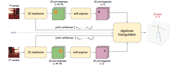
Figure 1. Outline of the approach based on algebraic triangulation with learned confidences. The input for the method is a set of RGB images with known camera parameters. The 2D backbone produces the joints’ heatmaps and camera-joint confidences. The 2D positions of the joints are inferred from 2D joint heatmaps by applying soft-argmax. The 2D positions together with the confidences are passed to the algebraic triangulation module that outputs the triangulated 3D pose. All blocks allow backpropagation of the gradients, so the model can be trained end-to-end.

In the algebraic triangulation baseline we process each joint \(j\) independently of each other.
The approach is built upon triangulating the 2D positions obtained from the j-joint’s backbone heatmaps from different views: \(H_{c,j} = h_{\theta}(I_c)_j\) (Figure 1).
To estimate the 2D positions we first compute the softmax across the spatial axes: \(H^{'}_{c,j} = \exp(\alpha H_{c,j})/ \sum^W_{r_x=1} \sum^H_{r_y=1} \exp(\alpha H_{c,j}(r))), \; \; \; (1)\)

where parameter \(\alpha\) is discussed below.
Then we calculate the 2D positions of the joints as the center of mass of the corresponding heatmaps (so-called soft-argmax operation): \[\mathrm{x}_{c,j} = \sum^W_{r_x=1} \sum^H_{r_y=1} \mathbf{r} \cdot (H^{'}_{c,j}(\mathbf{r})), \; \; \; (2)\]

An important feature of soft-argmax is that rather than getting the index of the maximum, it allows the gradients to flow back to heatmaps \(H_c\) from the output 2D position of the joints \(\mathrm{x}\).
Since the backbone was pretrained using a loss other than soft-argmax (MSE over heatmaps without softmax [16]), we adjust the heatmaps via multiplying them by an ’inverse temperature’ parameter \(\alpha = 100\) in (1), so at the start of the training the soft-argmax gives an output close to the positions of the maximum.

To infer the 3D positions of the joints from their 2D estimates \(\mathrm{x}_{c,j}\) we use a linear algebraic triangulation approach [1].
The method reduces the finding of the 3D coordinates of a joint \(y_j\) to solving the overdetermined system of equations on homogeneous 3D coordinate vector of the joint \(\tilde{y}\):
\(A_{j}\tilde{\mathrm{y}}_j = 0 \; \; \; (3)\)

where \(A_j \in \mathbb{R}^{(2C,4)}\) is a matrix composed of the components from the full projection matrices and \(x_{c,j}\) (see [1] for full details).

A naive triangulation algorithm assumes that the joint coordinates from each view are independent of each other and thus all make comparable contributions to the triangulation.
However, on some views the 2D position of the joints cannot be estimated reliably (e.g. due to joint occlusions), leading to unnecessary degradation of the final triangulation result.

This greatly exacerbates the tendency of methods that optimize algebraic reprojection error to pay uneven attention to different views.
The problem can be dealt with by applying RANSAC together with the Huber loss (used to score reprojection errors corresponding to inliers).
However, this has its own drawbacks.
E.g. using RANSAC may completely cut off the gradient flow to the excluded cameras.

To address the aforementioned problems, we add learnable weights \(w_c\) to the coefficients of the matrix corresponding to different views: \[(\mathbf{w}_j \circ A_j)\tilde{\mathrm{y}}_j = 0, \; \; \; (4)\]

where \(\mathbf{w}_j = (w_{1,j}, w_{1,j}, w_{2,j}, w_{2,j} , ... ,, w_{C,j} ,w_{C,j}); \circ\) denotes the Hadamard product (i.e. i-th row of matrix A is multiplied by i-th element of vector \(\mathbf{w}\)).
The weights \(w_{c,j}\) are estimated by a convolutional network \(q^{\phi}\) with learnable parameters \(\phi\) (comprised of two convolutional layers, global average pooling and three fully-connected layers), applied to the intermediate output of the backbone: \[w_{c,j} = (q^{\phi}(g^{\theta}(I_c)))_j \; \; \; (5)\]

This allows the contribution of the each camera view to be controlled by the neural network branch that is learned jointly with the backbone joint detector.

The equation (4) is solved via differentiable Singular Value Decomposition of the matrix \(B = UDV^T\) , from which \(\tilde{\mathrm{y}}\) is set as the last column of V.
The final nonhomogeneous value of \(\tilde{\mathrm{y}}\) is obtained by dividing the homogeneous 3D coordinate vector \(\tilde{\mathrm{y}}\) by its fourth coordinate: \(\mathrm{y} = \tilde{\mathrm{y}}/(\tilde{\mathrm{y}})_4\).

Volumetric triangulation approach.

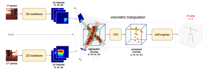
Figure 2. Outline of the approach based on volumetric triangulation. The input for the method is a set of RGB images with known camera parameters. The 2D backbone produces intermediate feature maps that are unprojected into volumes with subsequent aggreagation to a fixed size volume. The volume is passed to a 3D convolutional neural network that outputs the interpretable 3D heatmaps. The output 3D positions of the joints are inferred from 3D joint heatmaps by computing soft-argmax. All blocks allow backpropagation of the gradients, so the model can be trained end-to-end.

The main drawback of the baseline algebraic triangulation approach is that the images \(I_c\) from different cameras are processed independently from each other, so there is no easy way to add a 3D human pose prior and no way to filter out the cameras with wrong projection matrices.

To solve this problem we propose to use a more complex and powerful triangulation procedure.
We unproject the feature maps produced by the 2D backbone into 3D volumes (see Figure 2).
This is done by filling a 3D cube around the person via projecting output of the 2D network along projection rays inside the 3D cube.
The cubes obtained from multiple views are then aggregated together and processed.
For such volumetric triangulation approach, the 2D output does not have to be interpretable as joint heatmaps, thus, instead of unprojecting \(H_c\) themselves, we use the output of a trainable single layer convolutional neural network \(o^{\gamma}\) with \(1 \times 1\) kernel and \(\mathrm{K}\) output channels (the weights of this layer are denoted by \(\gamma\)) applied to the input from the backbone intermediate heatmaps \(f^{\theta}(I_c)\): \[M_{c,k} = o^{\gamma}(f^{\theta}(I_c))_k \; \; \; (6)\]

To create the volumetric grid, we place a \(L \times L \times L\) - sized 3D bound box in the global space around the human pelvis (the position of the pelvis is estimated by the algebraic triangulation baseline described above, \(L\) denotes the size of the box in meters) with the Y-axis perpendicular to the ground and a random orientation of the X-axis.
We discretize the bounding box by a volumetric cube \(V^{coords} \in \mathbb{R}^{64,64,64,3}\), filling it with the global coordinates of the center of each voxel (in a similar way to [5]).

For each view, we then project the 3D coordinates in \(V^{coords}\) to the plane: \(V^{proj}_c = P_cV^{coords}\) (note that \(V^{proj}_c \in \mathbb{R}^{64,64,64,2}\) ) and fill a cube \(V^{view}_c \in \mathbb{R}^{64,64,64,K}\) by bilinear sampling [4] from the maps \(M_{c,k}\) of the corresponding camera view using 2D coordinates in \(V^{proj}_c\) : \[V^{view}_{c,k} = M_{c,k}\{V^{proj}_c\}, \; \; \; \; (7)\]

where \(\{ \cdot \}\) denotes bilinear sampling.
We then aggregate the volumetric maps from all views to form an input to the further processing that does not depend on the number of camera views.
We study three diverse methods for the aggregation:

1. Raw summation of the voxel data: \(V^{input}_{k} = \sum_c V^{view}_{c,k}, \; \; \; \; (8)\)

2. Summation of the voxel data with normalized confidence multipliers \(d_c\) (obtained similarly to \(w_c\) using a branch attached to backbone): \(V^{input}_k = \sum_c(d_c \cdot V^{view}_{c,k}) / \sum_c d_c \; \; (9)\)

3. Calculating a relaxed version of maximum. Here, we first compute the softmax for each individual voxel \(V^{view}_c\) across all cameras, producing the volumetric coefficient distribution \(V^w_{c,k}\) with the role similar to scalars \(d_c\):

\[V_{c,k}^w = \exp(V^{view}_{c,k}) / \sum_c \exp(V^{view}_{c,k}) \; \; (10)\]

Then, the voxel maps from each view are summed with the volumetric coefficients \(V^w_c\) : \[V^{input}_k = \sum_c V^w_{c,k} \circ V^{view}_c \; \; \; (11)\]

Aggregated volumetric maps are then fed into a learnable volumetric convolutional neural network \(u^v\) (with weights denoted by \(v\)), with architecture similar to V2V [11], producing the interpretable 3D-heatmaps of the output joints: \[V^{output}_j = (u^v(V^{input}))_j \; \; \; (12)\]

Next, we compute softmax of \(V^{output}_j\) across the spatial axes (similar to (1)): \[V'^{output}_j = \exp(V^{output}_j) / (\sum^W_{r_x=1}\sum^H_{r_y=1}\sum^D_{r_z=1} \exp(V^{output}_j (\mathbf{r}))), \; \; \; (13)\]

and estimate the center of mass for each of the volumetric joint heatmaps to infer the positions of the joints in 3D: \[y_i = \sum^W_{r_x=1}\sum^H_{r_y=1}\sum^D_{r_z=1} \mathbf{r} \cdot V'^{output}_j(\mathbf{r}), \; \; \; (14)\]

Lifting to 3D allows getting more robust results, as the wrong predictions are spatially isolated from the correct ones inside the cube, so they can be discarded by convolutional operations.
The network also naturally incorporates the camera parameters (uses them as an input), allows modelling the human pose prior and can reasonably handle multimodality in 2D detections.

Losses.

For both of the methods described above, the gradients pass from the output prediction of 3D joints’ coordinates \(y_j\) to the input RGB-images \(I_c\) making the pipeline trainable end-to-end. For the case of algebraic triangulation, we apply a soft version of per-joint Mean Square Error (MSE) loss to make the training more robust to outliers. This variant leads to better results compared to raw MSE or L1 (mean absolute error):

Here, \(\varepsilon\) denotes the threshold for the loss, which is set to (20 cm)² in the experiments.
The final loss is the average over all valid joints and all scenes in the batch.

For the case of volumetric triangulation, we use the L1 loss with a weak heatmap regularizer, which maximizes the prediction for the voxel that has inside of it the ground-truth joint: \[\mathcal{L}^{vol}(\theta, \gamma, \nu) = \sum_j \vert y_j - y_j^{gt} \vert - \beta \cdot log(V_j^{output}(y^{gt}_j)) \; \; (16)\]

Without the second term, for some of the joints (especially, pelvis) the produced output volumetric heatmaps are not interpretable, probably due to insufficient size of the training datasets [16].
Setting the \(\beta\)to a small value (\(\beta = 0.01\)) makes them interpretable, as the produced heatmaps always have prominent maxima close to the prediction.
At the same time, such small \(\beta\) does not seem to have any effect on the final metrics, so its use can be avoided if interpretability is not needed.
We have also tried the loss (15) from the algebraic triangulation instead of L1, but it performed worse in our experiments.

4. Experiments

Human3.6M dataset.

CMU Panoptic dataset.

5. Conclusion

We have presented two novel methods for the multi-view 3D human pose estimation based on learnable triangulation that achieve state-of-the-art performance on the Human3.6M dataset.
The proposed solutions drastically reduce the number of views needed to achieve high accuracy, and produce smooth pose sequences on the CMU Panoptic dataset without any temporal processing (see our project page for demonstration), pointing that it can potentially improve the ground truth annotation of the dataset.
An ability to transfer the trained method between setups is demonstrated for the CMU Panoptic -> Human3.6M pair.
The volumetric triangulation strongly outperformed all other approaches both on CMU Panoptic and Human3.6M datasets.
We speculate that due to its ability to learn a human pose prior this method is robust to occlusions and partial views of a person.
Another important advantage of this method is that it explicitly takes the camera parameters as independent input.
Finally, volumetric triangulation also generalizes to monocular images if human’s approximate position is known, producing results close to state of the art.

One of the major limitations of our approach is that it supports only a single person in the scene.
This problem can be mitigated by applying available ReID solutions to the 2D detections of humans, however there might be more seamless solutions.
Another major limitation of the volumetric triangulation approach is that it relies on the predictions of the algebraic triangulation.
This leads to the need for having at least two camera views that observe the pelvis, which might be a problem for some applications.
The performance of our method can also potentially be further improved by adding multi-stage refinement in a way similar to [18].