Cross View Fusion for 3D Human Pose Estimation

Cross View Fusion for 3D Human Pose Estimation 요약

multi-view geometric priors들을 통합함으로써 multi-view images에서 absolute 3D human poses를 recovering

2개의 구별되는 steps으로 구성되어있다.
(1) multi-view images에서 2D poses를 추정
(2) multi-view 2D poses에서 3D poses를 복원

첫째, multiple views에서 2D pose를 jointly하게 estimate하기 위해 CNN에 cross-view fusion scheme를 도입하였다.
결론적으로, 각 view에서 2D pose estimation은 이미 다른 views로 부터 혜택을 얻는다.

둘째, multi-view 2D poses에서 3D pose를 recover하기 위해 재귀적 Pictorial Structure Model을 제시한다.
이것은 합리적인 계산 비용으로 정확한 3D pose를 점진적으로 개선한다.

본 논문은 multiple cameras에서 world coordinate system인 absolute 3D poses를 estimate하는 문제를 다룬다.

3D pose recovering 배경 지식 PSM 개념과 문제

3D pose를 recovering하는 것은 2D pose를 estimating하는 단계에서 image에 occlusion이나 motion blur가 있을때 large error를 갖는다.
-> Pictorial Structure Model (PSM)을 3D pose estimation에 사용하는것은 spatial dependence(공간 의존성)을 고려함으로써 부정확한 2D joints의 영향을 완화할수 있다.

Pictorial Structure Model (PSM)은 root joint 주위 공간을 \(N \times N \times N\) grid로 이산화하고 하나의 \(N^3\) bins에 각 joint를 할당한다 (hypotheses).
–> 이것은 estimated 3D pose와 2D pose간의 projection error를 jointly하게 최소화하고
–> joints의 spatial configuration(공간 구성)과 그것들의 prior structures의 불일치를 최소화한다.: 하지만 공간 이산화는 large quantization errors를 일으킨다.; \(N\)을 증가시킴으로써 error를 줄일 수 있지만 inference 비용이 \(O(N^6)\)만큼 증가한다.

##work flow

Fig1

첫번째, CNN based approach를 사용하여 multiple views로부터 jointly하게 estimating함으로써 더 정확한 2D poses를 얻는다.
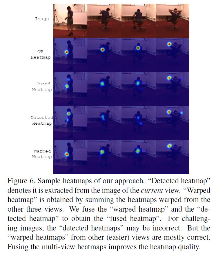
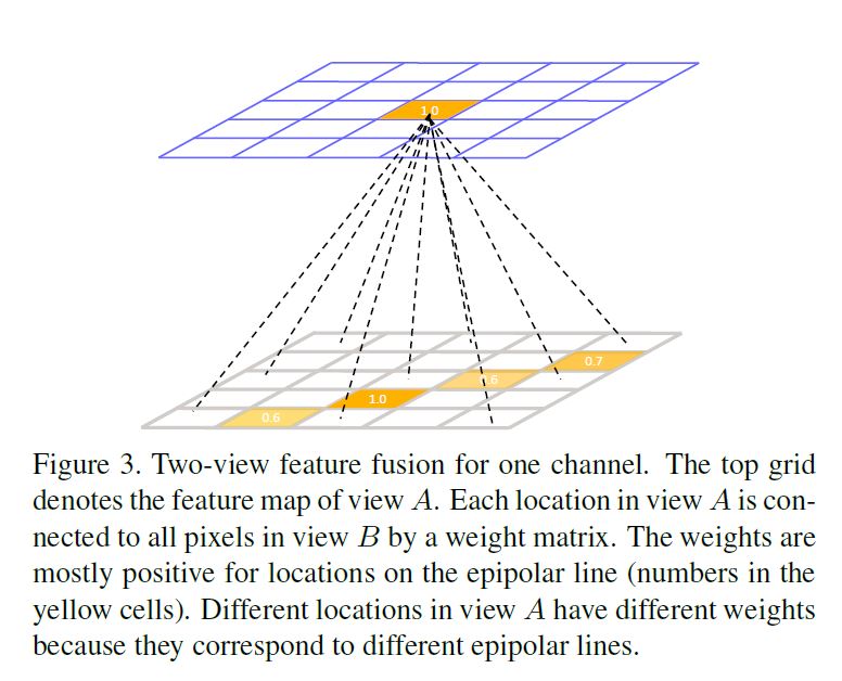
2D pose heatmap fusion을 위해 서로 다른 views들 사이에서 해당 위치를 찾아야 함 : fusion neural network를 통해 이것을 수행한다.

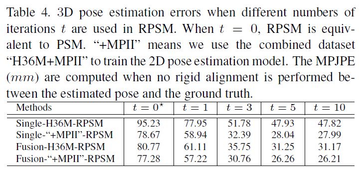
두번째, estimated된 multiview 2D pose heatmaps으로부터 3D pose를 recover하기 위해, Recursive Pictorial Structure Model (RPSM)를 제시한다.
quantization error를 제어하기 위해 공간의 많은 수의 bins로 직접 분리하는 PSM과 달리, RPSM은 적은 수의 bins을 사용하여 각 joint 위치 주변의 공간을 보다 세분화된(finer-grained) grid로 재귀적으로 분리한다.
결과적으로 estimated된 3D pose는 step by step으로 refine된다.

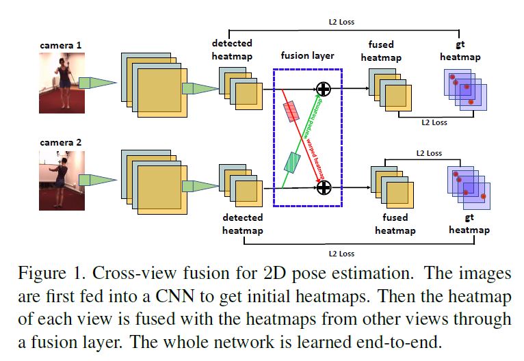
Cross View Fusion for 2D Pose Estimation

2D Pose Estimation에 대한 Cross View Fusion

논문의 2D pose estimator는 multi-view images를 input으로 한다.
각각을 초기 initial pose heatmaps를 생성하고 그런 다음 각 view의 heatmap이 다른 views로 부터 이득을 얻는것 처럼 다른 views들에 걸처 heatmaps들을 fuse한다.: 우리의 fusion approach의 핵심은 views들의 pair간의 corresponding한 features들을 찾는것이다.

Fig2

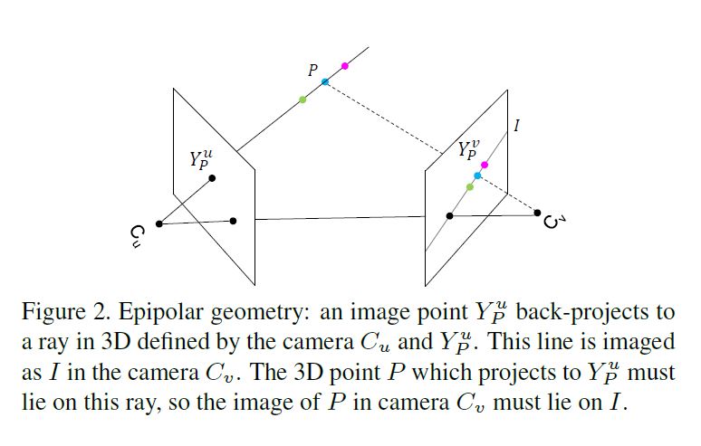
3D point \(P\)를 view u의 \(Z^u\)평면위의 점 \(Y^u_P\)만 알고 있다고 가정하면, 이것에 corresponding한 다른 view image의 point \(Y^v_P\)를 어떻게 찾을 수 있을까?
\(Y_P^v\)가 epipolar line \(I\)위에 놓여있음을 알고 있다.
3D point \(P\)는 \(C_u\)와 \(Y^u_P\)를 잇는 선에 있다는것을 알지만 \(P\)의 depth를 모르기 때문에 \(P\)는 \(C_u\)와 \(Y^u_P\)위에서 움직이며 때문에 Epipolar line \(I\) 위에 \(Y^v_P\)의 정확한 location을 결정할수 없다.: 이런 모호성이 cross view fusion의 어려움준다.

본 논문의 solution은 epipolar line \(I\)위의 모든 features와 point \(Y^u_P\)의 feature \(x^u_i\)를 fuse하는것이다.
즉 heatmap layer의 fusion은 \(x^u_i\)에 상응하는 \(x^v_j\)는 \(Y^v_P\)에 large reponse를 가져야 한다.

epipolar line \(I\)가 아닌 다른 위치는 0, 즉 non-corresponding한 위치는 기여하지 않고 fusion도 거의 일어나지 않는다.
따라서 epipolar line위의 모든 pixels를 fusing하는것은 간단하지만 효과적인 solution이다.

Fig3

Limitation and Solution

epipolar geometry의 정보를 암시적으로 encode하는 학습된 fusion weights는 camera configurations에 따라 달라진다.
결과적으로 특정 camera configuration에서 train된 model은 다른 configuration에 직접 적용할수 없다.

본 논문은 어떠한 annotations 없이 새로운 환경에 논문의 model이 자동적으로 적용되는 approach를 제안한다.
본 논문는 [21]과 같이 semi-supervised training approach를 채택한다.

학습
ground truth pose annotations을 가지고 있는 MPII와 같은 이미 존재하는 datasets에 single view 2D pose estimator를 train한다.
그런다음 우리는 trained model을 새로운 환경에서 multiple cameras에 의헤 얻은 images에 적용하고 poses의 set을 pseudo labels로 수확한다.
몇몇 이미지에서 estimations가 정확하지 않기 때문에, multi-view consistency로 incorrect labels를 거르는것을 제안한다.

3D Pose Estimation 설명

PSM for Multi-view 3D Pose Estimation

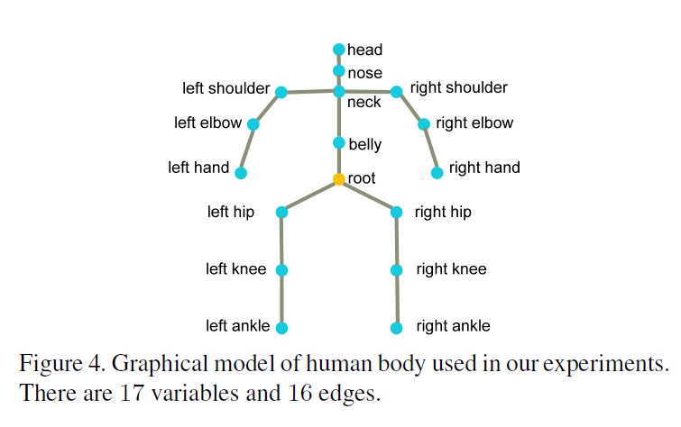
body joint에 대응되는 각 variable로 이루어진 random variables \(\mathcal{J} = \{J_1,…,J_M\}\)으로 human body를 graphical model로 나타낸다.
각 variable \(J_i\)는 state vector \(J_i= [x_i,y_i,z_i]\) 를 body joint를 world coordinate system의 3D position으로 정의한다.
2개의 variables간의 edge는 2개의 variables의 conditional dependence(조건 의존성)을 나타낸다. 그리고 physical constraint(물리적 제약)으로 해석된다.

Pictorial Structure Model

Given 3D pose의 configuration \(\mathcal{J}\)와 multi-view 2D pose heatmaps \(\mathcal{F}\), posterior :
\(p(\mathcal{J} \vert \mathcal{F})= \frac{1}{Z(\mathcal{F})} ∏_{i=1}^M ϕ_i^{conf} (J_i,\mathcal{F}) ∏_{(m,n)∈ε}ψ^{limb} (J_m,J_n)\) (Eq.(2))
\(Z(\mathcal{F})\) : partition function \(ε\) : graph edges
unary potential functions \(∅_i^{conf} (J_i,\mathcal{F})\)은 previously estimated mulit-view 2D pose heatmaps \(\mathcal{F}\)을 기반으로 계산된다.
pairwise potential functions \(ψ^{limb} (J_m,J_n)\)은 joints간 limb length constraints를 encode한다.

Discrete state space (상태 공간 이산화) 먼저 모든 views에서 detected된 2D locations를 사용하여 root joint의 3D location을 triangulate한다.
그리고 3D pose의 state space는 root joint를 중심으로 3D bounding volume안에 있게 된다.

Unary potentials 모든 body joint hypothesis(즉 grid \(\mathcal{G}\)의 bin)은 3D position in the world coordinate system.
우리는 이것을 camera parameters를 사용하여 모든 camera views의 pixel coordinate system에 project한다, 그리고 상응하는 \(\mathcal{F}\)의 joint confidence를 얻는다. hypothesis을 위한 unary potential로서 모든 camera views의 평균 confidence를 계산한다.

Pairwise potentials edge set \(ε\)에 대해 joints들의 각 pair \((J_m,J_n)\), training set에서 평균 거리 \(l_(m,n)\)을 limb length priors로 계산한다.

inference동안, pairwise potential은 다음과 같이 정의된다.
\(l_{m,n}\) 이 \(l_{m,n}\) 의 평균 값 ± \(ϵ\) 이 값 이내면 1, 아님 0.
\(l_{m,n}\) 은 \(J_m\) and \(J_n\)사이의 거리값. pairwise term은 3D poses가 합리적인 limb lengths를 가지게 한다.

Inference 최종 단계는 discrete state space에 (Eq.(2)) posterior을 maximize하는것이다. graph가 비순환구조이기 때문에 global optimum guarantee로 dynamic programming에 의해 optimized될 수 있다. 계산 복잡성은 \(O(N^6)\)

Fig4

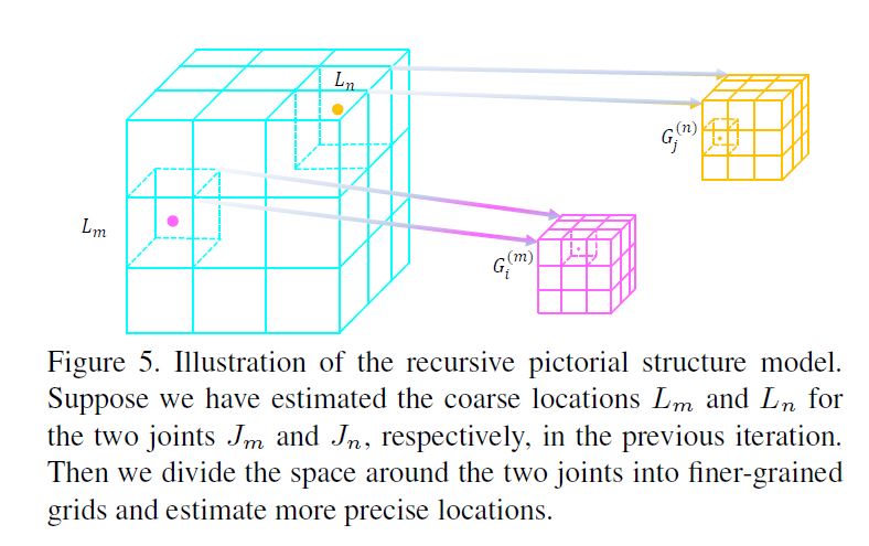
Recursive Pictorial Structure Model

Fig5

PSM model은 space discretization으로 발생하는 large quantization errors을 겪는다. \(N\)을 늘리면 quantization error를 줄일수 있지만 computation time은 빠르게 다루기 힘들어진다 즉 느려진다.

한 iteration에 large N을 사용하는것 대신 multiple stage process를 통해 joint locations을 recursively하게 refine하는 것을 제안한다.
그리고 각 stage별 small N을 사용하는것을 제안한다.

first stage(t=0)에서 coarse(거친) grid (\(N=16\))를 이용하여 triangulated된 root joint 주위의 3D bounding volume space를 discretize한다.

PSM approach를 사용하여 초기 3D pose estimation \(L = (L_1,· · · ,L_M )\)을 얻는다.
계속해서 다음 stages들부터(t ≥ 1), 각 joint \(J_i\)에서, 우리는 현재 location \(L_i\) 주변의 space를 \(2 \times 2 \times 2\) grid \(G^{(i)}\)로 discretize한다. (Figure5 참고)

여기서 space discretization은 PSM과 2가지면에서 다르다.

첫째, different joints는 그들 자신의 grids를 갖지만, PSM에서는 모든 joints들이 같은 grid를 공유한다.
두번째, bounding volume의 edge length는 iterations돌때마다 줄어드는데 이것은 이전 stage와 비교하여 grid가 finer-grained되는 주요 이유이다.
각 joint를 독립적으로 refining하는 대신에, 우리는 동시에 spatial relations를 고려하여 모든 joints를 refine한다.

center locations, sizes, the number of bins of the grids를 알고있다, 따라서 우린는 unary potentials와 pairwise potentials를 계산할수 있어 grids에 모든 bin의 위치를 계산할수 있다.
pairwise potentials는 이전 estimated된 locations에 따라 달라지기 때문에 이것을 즉시 계산해야한다. 그러나 우리는 \(N\)을 작은 값으로 설정했기 때문에 이 계산은 빠르다

Table1