ICLR 2017 paper

Dan Hendrycks
University of California, Berkeley

Kevin Gimpel
Toyota Technological Institute at Chicago

ABSTRACT

We consider the two related problems of detecting if an example is misclassified or out-of-distribution.
We present a simple baseline that utilizes probabilities from softmax distributions.
Correctly classified examples tend to have greater maximum softmax probabilities than erroneously classified and out-of-distribution examples, allowing for their detection.
We assess performance by defining several tasks in computer vision, natural language processing, and automatic speech recognition, showing the effectiveness of this baseline across all.
We then show the baseline can sometimes be surpassed, demonstrating the room for future research on these underexplored detection tasks.

우리는 example이 misclassified되었거나 out-of-distribution인 경우 detecting하는 두 가지 관련 문제를 고려한다.
우리는 softmax distributions의 probabilities을 활용하는 simple baseline을 제시한다.
Correctly classified examples는 detection에서 erroneously classified와 out-of-distribution examples보다 maximum softmax probabilities이 더 큰 경향이 있다.
우리는 컴퓨터 비전, 자연어 처리 및 자동 음성 인식에서 여러 작업을 정의하고 성능을 평가하여 이 baseline의 전반적인 효과를 보여준다.
그런 다음 때로는 baseline이 능가할 수 있음을 보여 주며, 이러한 underexplored detection tasks에 대한 향후 연구의 여지를 보여준다.

INTRODUCTION

When machine learning classifiers are employed in real-world tasks, they tend to fail when the training and test distributions differ.
Worse, these classifiers often fail silently by providing high-confidence predictions while being woefully incorrect (Goodfellow et al., 2015; Amodei et al., 2016).
Classifiers failing to indicate when they are likely mistaken can limit their adoption or cause serious accidents.
For example, a medical diagnosis model may consistently classify with high confidence, even while it should flag difficult examples for human intervention.
The resulting unflagged, erroneous diagnoses could blockade future machine learning technologies in medicine.
More generally and importantly, estimating when a model is in error is of great concern to AI Safety (Amodei et al., 2016).

machine learning classifiers가 real-world tasks에 사용될 때, training distributions과 test distributions가 다를 때 실패하는 경향이 있다.
더 나쁜 것은, 이러한 classifiers가 비정상적으로 부정확한 상태에서 높은 신뢰도 예측을 제공함으로써 조용히 실패하는 경우가 많다는 것이다(Goodfellow et al., 2015; Amodei et al., 2016).
Classifiers가 잘못될 가능성이 있을 떄를 표시하지 않으면 채택이 제한되거나 심각한 사고를 유발할 수 있다.
예를 들어, 의료 진단 모델은 인간의 개입을 위한 어려운 examples를 flag해야 하지만 높은 신뢰도로 일관되게 분류할 수 있다.
그 결과로 unflagged된, 잘못된 진단은 의학에서 미래의 machine learning 기술을 차단할 수 있다.
보다 일반적으로 그리고 중요하게, 모델이 오류에 있는 시점을 추정하는 것이 AI Safety에 큰 관심사이다(Amodei et al., 2016).

These high-confidence predictions are frequently produced by softmaxes because softmax probabilities are computed with the fast-growing exponential function.
Thus minor additions to the softmax inputs, i.e. the logits, can lead to substantial changes in the output distribution.
Since the softmax function is a smooth approximation of an indicator function, it is uncommon to see a uniform distribution outputted for out-of-distribution examples.
Indeed, random Gaussian noise fed into an MNIST image classifier gives a “prediction confidence” or predicted class probability of 91%, as we show later.
Throughout our experiments we establish that the prediction probability from a softmax distribution has a poor direct correspondence to confidence.
This is consistent with a great deal of anecdotal evidence from researchers (Nguyen & O’Connor, 2015; Yu et al., 2010; Provost et al., 1998; Nguyen et al., 2015).

softmax probabilities은 빠르게 증가하는 exponential function로 계산되기 때문에, 이러한 높은 신뢰도 예측은 softmaxes에 의해 자주 생성된다.
따라서 softmax inputs, 즉 logits에 대한 minor additions는 output distribution에 상당한 변화를 가져올 수 있다.
softmax function은 indicator function의 smooth 근사치이기 때문에, out-of-distribution examples를 출력하는 uniform distribution를 보는 것은 드문 일이다.
실제로, MNIST image classifier에 공급되는 random Gaussian noise는 나중에 우리가 보여주듯이 “prediction confidence(예측 신뢰도)” 또는 91%의 예측된 class probability를 제공한다.
실험을 통해 우리는 softmax distribution의 prediction probability이 confidence와 직접 일치하지 않음을 확인한다.
이는 연구자들의 많은 입증되지 않은 증거와 일치한다(Nguyen & O’Connor, 2015; Yu et al., 2010; Provost et al., 1998; Nguyen et al., 2015).

However, in this work we also show the prediction probability of incorrect and out-of-distribution examples tends to be lower than the prediction probability for correct examples.
Therefore, capturing prediction probability statistics about correct or in-sample examples is often sufficient for detecting whether an example is in error or abnormal, even though the prediction probability viewed in isolation can be misleading.

그러나 본 연구에서는 incorrect examples와 out-of-distribution examples의 예측 확률이 correct examples의 예측 확률보다 낮은 경향이 있음을 보여준다.
따라서, correct or in-sample examples에 대한 예측 확률 통계를 캡처하는 것은 example이 error인지 abnormal인지 여부를 detecting하는 데 충분하지만, isolation하여 보는 예측 확률은 misleading할수 있다.

These prediction probabilities form our detection baseline, and we demonstrate its efficacy through various computer vision, natural language processing, and automatic speech recognition tasks.
While these prediction probabilities create a consistently useful baseline, at times they are less effective, revealing room for improvement.
To give ideas for future detection research, we contribute one method which outperforms the baseline on some (but not all) tasks.
This new method evaluates the quality of a neural network’s input reconstruction to determine if an example is abnormal.

이러한 예측 확률은 우리의 detection baseline을 형성하며, 다양한 컴퓨터 비전, 자연어 처리, 자동 음성 인식 작업을 통해 그 효과를 입증한다.
이러한 예측 확률은 지속적으로 유용한 baseline을 생성하지만 때로는 덜 효과적이어서 개선의 여지가 있다.
향후 detection research를 위한 아이디어를 제공하기 위해, 우리는 일부 (전부는 아니지만) 작업의 baseline을 능가하는 한 가지 방법을 제안한다.
이 새로운 방법은 신경망의 input reconstruction의 quality를 평가하여 example가 abnormal인지 여부를 결정한다.

In addition to the baseline methods, another contribution of this work is the designation of standard tasks and evaluation metrics for assessing the automatic detection of errors and out-of-distribution examples.
We use a large number of well-studied tasks across three research areas, using standard neural network architectures that perform well on them.
For out-of-distribution detection, we provide ways to supply the out-of-distribution examples at test time like using images from different datasets and realistically distorting inputs.
We hope that other researchers will pursue these tasks in future work and surpass the performance of our baselines.

baseline methods 외에도, 이 작업의 또 다른 contribution은 errors의 automatic detection과 out-of-distribution examples를 평가하기 위한 standard tasks 및 evaluation metrics을 설계하였다.
우리는 세 가지 연구 분야에 걸쳐 잘 연구된 많은 tasks을 사용하는데, 그 tasks에 잘 작용하는 standard neural network architectures를 사용한다.
out-of-distribution detection를 위해, 우리는 다른 datasets의 이미지를 사용하는 것과 input data가 현실적으로 왜곡되는 것과 같은 out-of-distribution examples를 제공할 수 있는 방법을 제공한다.
우리는 다른 연구자들이 향후 작업에서 이러한 과제를 추구하고 우리의 baselines의 performance를 능가하기를 바란다.

In summary, while softmax classifier probabilities are not directly useful as confidence estimates, estimating model confidence is not as bleak as previously believed.
Simple statistics derived from softmax distributions provide a surprisingly effective way to determine whether an example is misclassified or from a different distribution from the training data, as demonstrated by our experimental results spanning computer vision, natural language processing, and speech recognition tasks.
This creates a strong baseline for detecting errors and out-of-distribution examples which we hope future research surpasses.

요약하자면, softmax classifier probabilities는 신뢰 추정치만큼 직접적으로 유용하지는 않지만, 모델 신뢰 추정은 이전에 믿었던 것만큼 암울하지 않다.
softmax distributions에서 파생된 Simple statistics는 ,컴퓨터 비전, 자연어 처리 및 음성 인식 작업에 걸친 우리의 실험 결과에서 입증된 바와 같이, example이 misclassified되었는지 또는 training data와 다른 distribution에서 나온 것인지를 결정하는 놀랄 만큼 효과적인 방법을 제공한다.
이것은 우리가 향후 연구가 능가하기를 희망하는 errors와 out-of-distribution examples를 detecting하는 strong baseline을 만든다.

2 PROBLEM FORMULATION AND EVALUATION

In this paper, we are interested in two related problems.
The first is error and success prediction: can we predict whether a trained classifier will make an error on a particular held-out test example; can we predict if it will correctly classify said example?
The second is in- and out-of-distribution detection: can we predict whether a test example is from a different distribution from the training data; can we predict if it is from within the same distribution?
Below we present a simple baseline for solving these two problems.
To evaluate our solution, we use two evaluation metrics.

본 논문에서는 두 가지 문제에 관심을 가지고 있다.
첫 번째는 error와 success prediction:
우리는 훈련된 classifier가 특정 지연 test example에서 error를 만들지 예측할 수 있는가; 우리는 classifier가 해당 example를 정확하게 분류할지 예측할 수 있는가?
두 번째는 in- and out-of-distribution detection:
test example이 training data와 다른 distribution에서 나온 것인지 예측할 수 있는가; same distribution에서 나온 것인지 예측할 수 있는가?
아래에서 우리는 이 두 가지 문제를 해결하기 위한 simple baseline을 제시한다.
solution을 평가하기 위해 우리는 두 가지 evaluation metrics를 사용한다.

Before mentioning the two evaluation metrics, we first note that comparing detectors is not as straightforward as using accuracy.
For detection we have two classes, and the detector outputs a score for both the positive and negative class.
If the negative class is far more likely than the positive class, a model may always guess the negative class and obtain high accuracy, which can be misleading (Provost et al., 1998).
We must then specify a score threshold so that some positive examples are classified correctly, but this depends upon the trade-off between false negatives (fn) and false positives (fp).

두 가지 evaluation metrics를 언급하기 전에, 먼저 detectors를 비교하는 것이 accuracy를 사용하는 것만큼 간단하지 않다는 점에 알아야한다.
detection을 위해 우리는 두 개의 클래스를 가지고 있으며, detector는 positive class와 negative class 모두에 대한 score를 출력한다.
negative class가 positive class보다 훨씬 가능성이 높은 경우, 모델은 항상 negative class를 추측하고 높은 정확도를 얻을 수 있으며, 이는 misleading할 수 있다(Provost et al., 1998).
그런 다음 일부 positive examples가 올바르게 분류되도록 score threshold을 지정해야 하지만, 이는 false negatives(fn)와 false positives(fp) 사이의 trade-off에 따라 달라진다.

Faced with this issue, we employ the Area Under the Receiver Operating Characteristic curve (AUROC) metric, which is a threshold-independent performance evaluation (Davis & Goadrich, 2006).
The ROC curve is a graph showing the true positive rate (tpr = tp/(tp + fn)) and the false positive rate (fpr = fp/(fp + tn)) against each other.
Moreover, the AUROC can be interpreted as the probability that a positive example has a greater detector score/value than a negative example (Fawcett, 2005).
Consequently, a random positive example detector corresponds to a 50% AUROC, and a “perfect” classifier corresponds to 100%.

이 문제에 직면하여, 우리는 threshold-independent performance evaluation인 Area Under the Receiver Operating Characteristic curve (AUROC) metric을 사용한다(Davis & Goadrich, 2006).
ROC curve은 true positive rate (tpr = tp/(tp + fn))과 false positive rate (fpr = fp/(fp + tn))을 서로 비교하는 graph이다.
또한 AUROC는 positive example가 negative example보다 detector score/value가 더 클 확률로 해석될 수 있다(Fawcett, 2005).
따라서 random positive example detector는 50% AUROC에 해당하고 “perfect” classifier는 100%에 해당한다.

The AUROC sidesteps the issue of threshold selection, as does the Area Under the Precision-Recall curve (AUPR) which is sometimes deemed more informative (Manning & Schutze, 1999).
This is because the AUROC is not ideal when the positive class and negative class have greatly differing base rates, and the AUPR adjusts for these different positive and negative base rates.
For this reason, the AUPR is our second evaluation metric.
The PR curve plots the precision (tp=(tp+fp)) and recall (tp=(tp + fn)) against each other.
The baseline detector has an AUPR approximately equal to the precision (Saito & Rehmsmeier, 2015), and a “perfect” classifier has an AUPR of 100%.
Consequently, the base rate of the positive class greatly influences the AUPR, so for detection we must specify which class is positive.

AUROC는 때로 더 유익하다고 여겨지는 Area Under the Precision-Recall curve (AUPR)과 마찬가지로 threshold selection 문제를 회피한다(Maning & Schutze, 1999).
왜냐하면 AUROC는 positive class와 negative class가 크게 다른 base rates 가질 때 이상적이지 않고, AUPR은 이러한 서로 다른 positive 및 negative base rates에 대해 조정되기 때문이다.
이러한 이유로, AUPR은 우리의 두 번째 evaluation metric이다.
PR curve는 서로에 대한 precision(tp=(tp+fp)와 recall(tp=(tp+fn))을 plots한다.
baseline detector의 AUPR은 precision와 거의 동일하고(Saito & Rehmsmeier, 2015), “perfect” classifier의 AUPR은 100%이다.
결과적으로, positive class의 base rate는 AUPR에 크게 영향을 미치므로, detection를 위해 class가 positive임을 지정해야 한다.

In view of this, we show the AUPRs when we treat success/normal classes as positive, and then we show the areas when we treat the error/abnormal classes as positive.
We can treat the error/abnormal classes as positive by multiplying the scores by -1 and labeling them positive.
Note that treating error/abnormal classes as positive classes does not change the \(AUROC\) since if S is a score for a successfully classified value, and E is the score for an erroneously classified value, \(AUROC = P(S > E) = P(-E > -S)\).

이러한 관점에서, 우리는 success/normal classes를 positive으로 취급할 때, AUPR을 보여준 다음 error/abnormal classes를 positive으로 취급할 때, 영역을 보여준다.
우리는 점수를 -1로 곱하고 positive로 표시함으로써 error/abnormal classes를 positive의 classes로 처리할 수 있다.
S가 successfully classified value에 대한 score이고 E가 erroneously classified value에 대한 score인 경우, \(AUROC = P(S > E) = P(-E > -S)\) 이기 때문에 error/abnormal classes를 positive classes로 처리해도 \(AUROC\)는 변경되지 않는다.

We begin our experiments in Section 3 where we describe a simple baseline which uses the maximum probability from the softmax label distribution in neural network classifiers.
Then in Section 4 we describe a method that uses an additional, auxiliary model component trained to reconstruct the input.

우리는 Section 3에서 실험을 시작하여 neural network classifiers에서 softmax label distribution의 maximum probability을 사용하는 simple baseline을 설명한다.
그런 다음 Section 4에서는 입력을 재구성하기 위해 훈련된 additional, auxiliary model component를 사용하는 방법을 설명한다.

3 SOFTMAX PREDICTION PROBABILITY AS A BASELINE

In what follows we retrieve the maximum/predicted class probability from a softmax distribution and thereby detect whether an example is erroneously classified or out-of-distribution.
Specifically, we separate correctly and incorrectly classified test set examples and, for each example, compute the softmax probability of the predicted class, i.e., the maximum softmax probability.
From these two groups we obtain the area under PR and ROC curves.
These areas summarize the performance of a binary classifier discriminating with values/scores (in this case, maximum probabilities from the softmaxes) across different thresholds.
This description treats correctly classified examples as the positive class, denoted “Success” or “Succ” in our tables.
In “Error” or “Err” we treat the the incorrectly classified examples as the positive class; to do this we label incorrectly classified examples as positive and take the negatives of the softmax probabilities of the predicted classes as the scores.

이어지는 내용에서 우리는 softmax distribution에서 maximum/predicted class probability을 retrieve하고 example이 erroneously classified 또는 out-of-distribution인지 detect한다.
구체적으로, 우리는 correctly classified test set examples와 incorrectly classified test set examples를 분리하고, 각 example에 대해 predicted class의 softmax probability, 즉 maximum softmax probability을 계산한다.
이 두 그룹에서 PR 및 ROC curves 영역을 얻는다.
이러한 영역은 서로 다른 thresholds에 걸쳐 values/scores(이 경우 maximum probabilities from the softmaxes)를 구별하는 binary classifier의 성능을 summarize한다.
이 설명은 “Success” or “Succ”로 표시된, correctly classified examples들을 표에서 positive class로 하고
“Error” or “Err”로 표시된 incorrectly classified example들을 positive class로 취급한다; 이를 위해 우리는 incorrectly classified example들을 positive로 label하고 predicted classes의 softmax probabilities의 negatives을 scores로 받아들인다.

For “In,” we treat the in-distribution, correctly classified test set examples as positive and use the softmax probability for the predicted class as a score, while for “Out” we treat the out-of-distribution examples as positive and use the negative of the aforementioned probability.
Since the AUPRs for Success, Error, In, Out classifiers depend on the rate of positive examples, we list what area a random detector would achieve with “Base” values.
Also in the upcoming results we list the mean predicted class probability of wrongly classified examples (Pred Prob Wrong (mean)) to demonstrate that the softmax prediction probability is a misleading confidence proxy when viewed in isolation.
The “Pred. Prob (mean)” columns show this same shortcoming but for out-of-distribution examples.

“In”의 경우, 우리는 in-distribution, correctly classified test set examples를 positive로 처리하고 predicted class에 대한 softmax probability을 score로 사용하는 반면, “Out”의 경우 out-of-distribution examples를 positive로 처리하고 앞서 언급한 probability의 negative를 사용한다.
Success, Error, In, Out classifiers의 AUPR은 positive examples의 rate에 따라 달라지기 때문에, 우리는 random detector가 “Base” values으로 어떤 영역을 달성할지를 열거한다.
또한 다음 결과에서는 wrongly classified examples의 mean predicted class probability(Pred Prob Wrong (mean))을 나열하여 softmax prediction probability가 분리되어 볼 때 misleading confidence proxy임을 보여준다.
“Pred. Prob (mean)” columns은 동일한 shortcoming을 나타내지만 out-of-distribution examples를 나타냅니다.

Table labels aside, we begin experimentation with datasets from vision then consider tasks in natural language processing and automatic speech recognition.
In all of the following experiments, the AUROCs differ from the random baselines with high statistical significance according to the Wilcoxon rank-sum test.

Table labels과는 별도로, 우리는 vision에서 datasets를 사용한 실험을 시작한 다음 자연어 처리 및 자동 음성 인식의 작업을 고려한다.
다음 모든 실험에서, AUROCs는 Wilcoxon rank-sum test에 따라 통계적 의미(중요성,의의)가 높은 random baselines과 다르다.

3.1 COMPUTER VISION

In the following computer vision tasks, we use three datasets: MNIST, CIFAR-10, and CIFAR- 100 (Krizhevsky, 2009).
MNIST is a dataset of handwritten digits, consisting of 60000 training and 10000 testing examples.
Meanwhile, CIFAR-10 has colored images belonging to 10 different classes, with 50000 training and 10000 testing examples.
CIFAR-100 is more difficult, as it has 100 different classes with 50000 training and 10000 testing examples.

다음 computer vision tasks에서는 MNIST, CIFAR-10 및 CIFAR-100 (Krizhevsky, 2009)의 세 가지 datasets를 사용한다.
MNIST는 60000개의 training과 10000개의 testing examples로 구성된 손으로 쓴 숫자의 데이터 세트이다.
한편 CIFAR-10은 10개의 다른 classes에 속하는 컬러 이미지를 가지고 있으며, 5000개의 training과 10000개의 testing examples가 있다.
CIFAR-100은 50000개의 training과 10000개의 testing examples가 있는 100개의 다른 classes을 가지고 있기 때문에 더 어렵다.

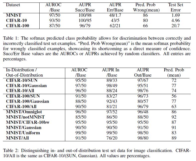
In Table 1, we see that correctly classified and incorrectly classified examples are sufficiently distinct and thus allow reliable discrimination.
Note that the area under the curves degrade with image recognizer test error.

표 1에서, 우리는 correctly classified examples들과 incorrectly classified examples들이 충분히 구별되므로 reliable discrimination을 허용함을 볼수 있다.
image recognizer test error로 인해 curves 아래의 영역이 저하된다.

Next, let us consider using softmax distributions to determine whether an example is in- or out-of-distribution.
We use all test set examples as the in-distribution (positive) examples.
For out-of-distribution (negative) examples, we use realistic images and noise.
For CIFAR-10 and CIFAR-100, we use realistic images from the ‘Scene UNderstanding dataset (SUN)’, which consists of 397 different scenes (Xiao et al., 2010).
For MNIST, we use grayscale realistic images from three sources.
Omniglot (Lake et al., 2015) images are handwritten characters rather than the handwritten digits in MNIST.
Next, notMNIST (Bulatov, 2011) consists of typeface characters.
Last of the realistic images, CIFAR-10bw are black and white rescaled CIFAR-10 images.
The synthetic “Gaussian” data is random normal noise, and “Uniform” data is random uniform noise.
Images are resized when necessary.

다음으로, softmax distributions를 사용하여 example이 in-of-distribution 인지 out-of-distribution 여부를 결정하는 것을 고려해본다.
in-distribution (positive) examples로 모든 test set examples를 사용한다.
out-of-distribution (negative) examples의 경우 현실적인 이미지와 노이즈를 사용한다.
CIFAR-10 및 CIFAR-100의 경우, 397개의 다른 장면으로 구성된 ‘Scene UNderstanding dataset (SUN)’의 실제 이미지를 사용한다(샤오 외, 2010).
MNIST의 경우, 세 가지 소스의 grayscale 실제 이미지를 사용한다.
Omniglot (Lake et al., 2015) 이미지는 MNIST에서 handwritten 숫자 대신 handwritten 문자이다.
다음으로, notMNIST (Bulatov, 2011) typeface characters로 구성된다.
마지막 실제 이미지인 CIFAR-10bw는 검은색과 흰색으로 재조정된 CIFAR-10 이미지이다.
synthetic “Gaussian” data는 random normal noise이며 “Uniform” data는 random uniform noise이다.
필요한 경우 이미지의 크기가 조정된다.

The results are shown in Table 2.
Notice that the mean predicted/maximum class probabilities (Pred. Prob (mean)) are above 75%, but if the prediction probability alone is translated to confidence, the softmax distribution should be more uniform for CIFAR-100.
This again shows softmax probabilities should not be viewed as a direct representation of confidence.
Fortunately, out-of-distribution examples sufficiently differ in the prediction probabilities from in-distribution examples, allowing for successful detection and generally high area under PR and ROC curves.

결과는 Table 2에 나와 있다.
mean predicted/maximum class probabilities (Pred. Prob (mean))는 75% 이상이지만 prediction probability만 confidence로 변환되면 CIFAR-100에 대해 softmax distribution가 더 uniform해야 한다.
이것은 softmax probabilities을 confidence의 직접적인 표현으로 간주해서는 안 된다는 것을 다시 보여준다.
다행히 out-of-distribution examples는 in-distribution examples와 예측 확률이 충분히 다르므로 성공적인 검출이 가능하고 일반적으로 PR 및 ROC 곡선에서 높은 area을 가질 수 있다.

For reproducibility, let us specify the model architectures.
The MNIST classifier is a three-layer, 256 neuron-wide, fully-connected network trained for 30 epochs with Adam (Kingma & Ba, 2015).
It uses a GELU nonlinearity (Hendrycks & Gimpel, 2016b), \(x\Phi(x)\), where \(\Phi(x)\) is the CDF of the standard normal distribution.
We initialize our weights according to (Hendrycks & Gimpel, 2016c), as it is suited for arbitrary nonlinearities.
For CIFAR-10 and CIFAR-100, we train a 40-4 wide residual network (Zagoruyko & Komodakis, 2016) for 50 epochs with stochastic gradient descent using restarts (Loshchilov & Hutter, 2016), the GELU nonlinearity, and standard mirroring and cropping data augmentation.

재현성을 위해 모델 아키텍처를 지정.
MNIST classifier는 three-layer, 256 neuron-wide, fully-connected, Adam, 30 epochs로 훈련된 network(Kingma & Ba, 2015)이다.
GELU nonlinearity (Hendrycks & Gimpel, 2016b), \(x\Phi(x)\)를 사용한다. 여기서 \(\Phi(x)\)는 CDF of the standard normal distribution이다.
임의의 비선형성에 적합하므로 (Hendryks & Gimpel, 2016c)에 따라 가중치를 초기화한다.
CIFAR-10 및 CIFAR-100의 경우, restarts (Loshchilov & Hutter, 2016), GELU nonlinearity, standard mirroring 및 cropping data augmentation을 사용하여 stochastic gradient descent을 가진 50 epochs에 대해 40-4 wide residual network (Zagoruyko & Komodakis, 2016)를 훈련한다.

3.2 NATURAL LANGUAGE PROCESSING

Let us turn to a variety of tasks and architectures used in natural language processing.

3.2.1 SENTIMENT CLASSIFICATION

The first NLP task is binary sentiment classification using the IMDB dataset (Maas et al., 2011), a dataset of polarized movie reviews with 25000 training and 25000 test reviews. This task allows us to determine if classifiers trained on a relatively small dataset still produce informative softmax distributions.
For this task we use a linear classifier taking as input the average of trainable, randomly initialized word vectors with dimension 50 (Joulin et al., 2016; Iyyer et al., 2015).
We train for 15 epochs with Adam and early stopping based upon 5000 held-out training reviews.
Again, Table 3 shows that the softmax distributions differ between correctly and incorrectly classified examples, so prediction probabilities allow us to detect reliably which examples are right and wrong.

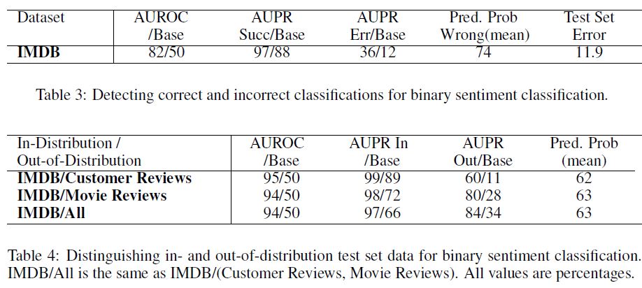
Now we use the Customer Review (Hu & Liu, 2004) and Movie Review (Pang et al., 2002) datasets as out-of-distribution examples.
The Customer Review dataset has reviews of products rather than only movies, and the Movie Review dataset has snippets from professional movie reviewers rather than full-length amateur reviews.
We leave all test set examples from IMDB as in-distribution examples, and out-of-distribution examples are the 500 or 1000 test reviews from Customer Review and Movie Review datasets, respectively. Table 4 displays detection results, showing a similar story to Table 2.

3.2.2 TEXT CATEGORIZATION

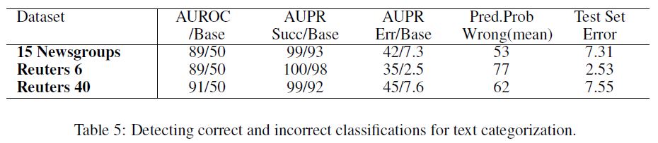
We turn to text categorization tasks to determine whether softmax distributions are useful for detecting similar but out-of-distribution examples.
In the following text categorization tasks, we train classifiers to predict the subject of the text they are processing.
In the 20 Newsgroups dataset (Lang, 1995), there are 20 different newsgroup subjects with a total of 20000 documents for the whole dataset.
The Reuters 8 (Lewis et al., 2004) dataset has eight different news subjects with nearly 8000 stories in total.
The Reuters 52 dataset has 52 news subjects with slightly over 9000 news stories; this dataset can have as few as three stories for a single subject.

For the 20 Newsgroups dataset we train a linear classifier on 30-dimensional word vectors for 20 epochs.
Meanwhile, Reuters 8 and Retuers 52 use one-layer neural networks with a bag-of-words input and a GELU nonlinearity, all optimized with Adam for 5 epochs.
We train on a subset of subjects, leaving out 5 newsgroup subjects from 20 Newsgroups, 2 news subjects from Reuters 8, and 12 news subjects from Reuters 52, leaving the rest as out-of-distribution examples.
Table 5 shows that with these datasets and architectures, we can detect errors dependably, and Table 6 informs us that the softmax prediction probabilities allow for detecting out-of-distribution subjects.

3.2.3 PART-OF-SPEECH TAGGING

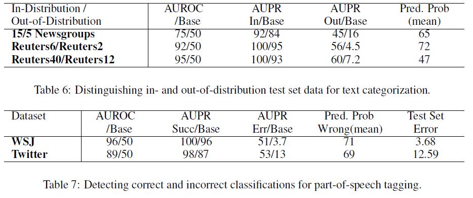
Part-of-speech (POS) tagging of newswire and social media text is our next challenge.
We use the Wall Street Journal portion of the Penn Treebank (Marcus et al., 1993) which contains 45 distinct POS tags.
For social media, we use POS-annotated tweets (Gimpel et al., 2011; Owoputi et al., 2013) which contain 25 tags.
For the WSJ tagger, we train a bidirectional long short-term memory recurrent neural network (Hochreiter & Schmidhuber, 1997) with three layers, 128 neurons per layer, with randomly initialized word vectors, and this is trained on 90% of the corpus for 10 epochs with stochastic gradient descent with a batch size of 32.
The tweet tagger is simpler, as it is twolayer neural network with a GELU nonlinearity, a weight initialization according to (Hendrycks & Gimpel, 2016c), pretrained word vectors trained on a corpus of 56 million tweets (Owoputi et al., 2013), and a hidden layer size of 256, all while training on 1000 tweets for 30 epochs with Adam and early stopping with 327 validation tweets.
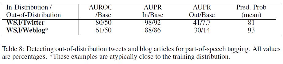
Error detection results are in Table 7. For out-ofdistribution detection, we use the WSJ tagger on the tweets as well as weblog data from the English Web Treebank (Bies et al., 2012).
The results are shown in Table 8. Since the weblog data is closer in style to newswire than are the tweets, it is harder to detect whether a weblog sentence is outof- distribution than a tweet.
Indeed, since POS tagging is done at the word-level, we are detecting whether each word is out-of-distribution given the word and contextual features.
With this in mind, we see that it is easier to detect words as out-of-distribution if they are from tweets than from blogs.

3.3 AUTOMATIC SPEECH RECOGNITION

Now we consider a task which uses softmax values to construct entire sequences rather than determine an input’s class.
Our sequence prediction system uses a bidirectional LSTM with two-layers and a clipped GELU nonlinearity, optimized for 60 epochs with RMSProp trained on 80% of the TIMIT corpus (Garofolo et al., 1993).
The LSTM is trained with connectionist temporal classification (CTC) (Graves et al., 2006) for predicting sequences of phones given MFCCs, energy, and first and second deltas of a 25ms frame.
When trained with CTC, the LSTM learns to have its phone label probabilities spike momentarily while mostly predicting blank symbols otherwise.
In this way, the softmax is used differently from typical classification problems, providing a unique test for our detection methods.

We do not show how the system performs on correctness/incorrectness detection because errors are not binary and instead lie along a range of edit distances.
However, we can perform out-of-distribution detection. Mixing the TIMIT audio with realistic noises from the Aurora-2 dataset (Hirsch & Pearce, 2000), we keep the TIMIT audio volume at 100% and noise volume at 30%, giving a mean SNR of approximately 5.
Speakers are still clearly audible to the human ear but confuse the phone recognizer because the prediction edit distance more than doubles.
For more out-of-distribution examples, we use the test examples from the THCHS-30 dataset (Wang & Zhang, 2015), a Chinese speech corpus.
Table 9 shows the results. Crucially, when performing detection, we compute the softmax probabilities while ignoring the blank symbol’s logit.
With the blank symbol’s presence, the softmax distributions at most time steps predict a blank symbol with high confidence, but without the blank symbol we can better differentiate between normal and abnormal distributions.
With this modification, the softmax prediction probabilities allow us to detect whether an example is out-of-distribution.

4 ABNORMALITY DETECTION WITH AUXILIARY DECODERS

Having seen that softmax prediction probabilities enable abnormality detection, we now show there is other information sometimes more useful for detection.
To demonstrate this, we exploit the learned internal representations of neural networks.
We start by training a normal classifier and append an auxiliary decoder which reconstructs the input, shown in Figure 1.
Auxiliary decoders are sometimes known to increase classification performance (Zhang et al., 2016).
The decoder and scorer are trained jointly on in-distribution examples.
Thereafter, the blue layers in Figure 1 are frozen.
Then we train red layers on clean and noised training examples, and the sigmoid output of the red layers scores how normal the input is.
Consequently, noised examples are in the abnormal class, clean examples are of the normal class, and the sigmoid is trained to output to which class an input belongs.
After training we consequently have a normal classifier, an auxiliary decoder, and what we call an abnormality module.
The gains from the abnormality module demonstrate there are possible research avenues for outperforming the baseline.

softmax prediction probabilities이 abnormality detection를 가능하게 한다는 것을 보고, 이제 우리는 때때로 detection에 더 유용한 다른 정보가 있음을 보여준다.
이를 입증하기 위해 신경망의 학습된 내부 표현(internal representations)을 활용한다.
우리는 normal classifier를 훈련시키는 것으로 시작하고 Figure 1에 나온 것처럼 입력을 재구성하는 보조 디코더(auxiliary decoder)를 추가한다.
보조 디코더(auxiliary decoder)는 때때로 분류 성능을 향상시키는 것으로 알려져 있다(Zhang et al., 2016).
디코더와 scorer는 in-distribution examples에 대해 공동으로 훈련된다.
그 후, Figure 1의 blue layers는 동결된다.
그런 다음 clean training examples하고 noised training examples에 대해 red layers를 훈련시키고, red layers의 sigmoid output는 입력이 얼마나 정상적인지를 점수화한다.
결과적으로, noised examples는 abnormal class에 있고, clean examples는 normal class에 속하며, sigmoid에는 입력이 속한 class에 출력하도록 훈련된다.
훈련 후에 우리는 결과적으로 normal classifier, auxiliary decoder, 그리고 우리가 abnormality module이라고 부르는 것을 갖게 된다.
abnormality module의 이득은 baseline을 능가할 수 있는 연구 방법이 있음을 보여준다.

4.1 TIMIT

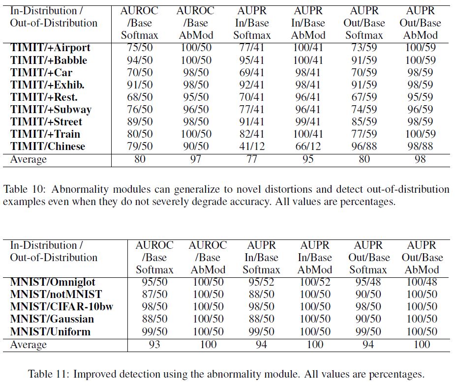
We test the abnormality module by revisiting the TIMIT task with a different architecture and show how these auxiliary components can greatly improve detection.
The system is a three-layer, 1024-neuron wide classifier with an auxiliary decoder and abnormality module.
This network takes as input 11 frames and must predict the phone of the center frame, 26 features per frame.
Weights are initialized according to (Hendrycks & Gimpel, 2016c).
This network trains for 20 epochs, and the abnormality module trains for two.
The abnormality module sees clean examples and, as negative examples, TIMIT examples distorted with either white noise, brown noise (noise with its spectral density proportional to \(1/f^2\)), or pink noise (noise with its spectral density proportional to \(1/f\)) at various volumes.

우리는 다른 아키텍처로 TIMIT 작업을 다시 방문하여 abnormality module을 테스트하고 이러한 auxiliary components가 detection을 크게 개선할 수 있는 방법을 보여준다.
이 시스템은 auxiliary decoder(보조디코더)와 abnormality module이 있는 1024-neuron wide classifier이다.
이 network는 input 11 frames으로 사용되며 frame당 26 features을 가진 center frame의 phone을 예측해야 한다.
가중치는 (Hendryks & Gimpel, 2016c)에 따라 초기화된다.
이 network는 20 epochs 동안 훈련하고, abnormality module은 2 epoch 동안 훈련한다.
abnormality module은 clean examples를 보고 negative examples로, 다양한 volumes에서 white noise, brown noise (noise with its spectral density proportional to \(1/f^2\)) 또는 pink noise (noise with its spectral density proportional to \(1/f\))로 왜곡된 TIMIT examples를 본다.

We note that the abnormality module is not trained on the same type of noise added to the test examples.
Nonetheless, Table 10 shows that simple noised examples translate to effective detection of realistically distorted audio.
We detect abnormal examples by comparing the typical abnormality module outputs for clean examples with the outputs for the distorted examples.
The noises are from Aurora-2 and are added to TIMIT examples with 30% volume.
We also use the THCHS-30 dataset for Chinese speech.
Unlike before, we use the THCHS-30 training examples rather than test set examples because fully connected networks can evaluate the whole training set sufficiently quickly.
It is worth mentioning that fully connected deep neural networks are noise robust (Seltzer et al., 2013), yet the abnormality module can still detect whether an example is out-of-distribution.
To see why this is remarkable, note that the network’s frame classification error is 29.69% on the entire test (not core) dataset, and the average classification error for distorted examples is 30.43%—this is unlike the bidirectional LSTM which had a more pronounced performance decline.
Because the classification degradation was only slight, the softmax statistics alone did not provide useful out-of-distribution detection.
In contrast, the abnormality module provided scores which allowed the detection of different-but-similar examples.
In practice, it may be important to determine whether an example is out-of-distribution even if it does not greatly confuse the network, and the abnormality module facilitates this.

abnormality module은 test examples에 추가된 동일한 유형의 노이즈에 대해 train되지 않는다.
그럼에도 불구하고 Table 10은 simple noised examples가 현실적으로 왜곡된 오디오의 효과적인 detection으로 해석된다는 것을 보여준다.
우리는 깨끗한 예제에 대한 일반적인 abnormality module outputs과 왜곡된 examples에 대한 outputs을 비교하여 abnormal examples를 감지한다.
이 noises은 Aurora-2에서 발생하며 30% 볼륨으로 TIMIT 예제에 추가됩니다.
또한 중국어 음성에는 THCS-30 데이터 세트를 사용한다.
이전과는 달리, 완전히 연결된 네트워크는 전체 훈련 세트를 충분히 빠르게 평가할 수 있기 때문에 테스트 세트 예보다는 THCs-30 훈련 예제를 사용한다.
완전히 연결된 심층 신경망은 노이즈가 강하지만(Seltzer et al., 2013) 이상 모듈은 여전히 예제가 분포 밖인지 여부를 감지할 수 있다는 것을 언급할 필요가 있다.
이것이 왜 주목할 만한지 알아보기 위해, 네트워크의 프레임 분류 오류는 전체 테스트(핵심이 아님) 데이터 세트에서 29.69%이고 왜곡된 예제의 평균 분류 오류는 30.43%이며, 이는 성능 저하가 더 두드러진 양방향 LSTM과는 다르다는 점에 유의한다.
분류 저하가 미미했기 때문에, 소프트맥스 통계만으로는 유용한 분포 외 탐지를 제공하지 못했다.
이와는 대조적으로, 이상 모듈은 서로 다르지만 유사한 예를 감지할 수 있는 점수를 제공했다.
실제적으로 예시가 네트워크를 크게 혼란시키지 않더라도 유통이 불가능한지를 판단하는 것이 중요할 수 있으며, 이상 모듈은 이를 촉진한다.

4.2 MNIST

Finally, much like in a previous experiment, we train an MNIST classifier with three layers of width 256.
This time, we also use an auxiliary decoder and abnormality module rather than relying on only softmax statistics.
For abnormal examples we blur, rotate, or add Gaussian noise to training images.
Gains from the abnormality module are shown in Table 11, and there is a consistent out-of-sample detection improvement compared to softmax prediction probabilities.
Even for highly dissimilar examples the abnormality module can further improve detection.

마지막으로, 이전 실험과 매우 유사하게, 우리는 width 256의 3 layers를 가진 MNIST classifier를 훈련시킨다.
이번에는 softmax statistics에만 의존하는 대신 auxiliary decoder와 abnormality module도 사용한다.
abnormal examples의 경우 훈련 이미지를 blur하거나 rotate하거나 Gaussian noise를 add한다.
abnormality module의 이득은 Table 11에 나타나 있으며, softmax prediction probabilities에 비해 일관된 out-of-sample detection 개선 효과가 있다.
매우 다른 예에서도 abnormality module은 detection을 더욱 향상시킬 수 있다.

5 DISCUSSION AND FUTURE WORK

The abnormality module demonstrates that in some cases the baseline can be beaten by exploiting the representations of a network, suggesting myriad research directions.
Some promising future avenues may utilize the intra-class variance: if the distance from an example to another of the same predicted class is abnormally high, it may be out-of-distribution (Giryes et al., 2015).
Another path is to feed in a vector summarizing a layer’s activations into an RNN, one vector for each layer.
The RNN may determine that the activation patterns are abnormal for out-of-distribution examples.
Others could make the detections fine-grained: is the out-of-distribution example a known-unknown or an unknown-unknown?
A different avenue is not just to detect correct classifications but to output the probability of a correct detection.
These are but a few ideas for improving error and out-of-distribution detection.

abnormality module은 network의 representations을 활용하여 수많은 연구 방향을 제시함으로써 어떤 경우에는 baseline을 이길 수 있음을 보여준다.
일부 유망한 미래 방법은 클래스 내 분산(intra-class variance)을 활용할 수 있다: same predicted class의 한 example에서 다른 example까지의 거리가 abnormally high하면, out-of-distribution일 수 있다(Giryes et al., 2015).
또 다른 path는 layer’s activations를 요약하는 벡터로 각 layer에 대해 하나의 벡터인 RNN으로 전달하는 것이다. RNN은 activation patterns이 out-of-distribution examples에 대해 abnormal이라고 판단할 수 있다.
다른 이들은 탐지 내용을 세분화(fine-grained)할 수 있다: out-of-distribution example가 known-unknown인지 unknown-unknown인지
다른 방법은 단지 정확한 분류를 감지하는 것이 아니라 정확한 검출의 확률을 출력하는 것이다.
이는 error 및 out-of-distribution detection을 개선하기 위한 몇 가지 아이디어에 불과하다.

We hope that any new detection methods are tested on a variety of tasks and architectures of the researcher’s choice.
A basic demonstration could include the following datasets: MNIST, CIFAR, IMDB, and tweets because vision-only demonstrations may not transfer well to other architectures and datasets.
Reporting the AUPR and AUROC values is important, and so is the underlying classifier’s accuracy since an always-wrong classifier gets a maximum AUPR for error detection if error is the positive class.
Also, future research need not use the exact values from this paper for comparisons.
Machine learning systems evolve, so tethering the evaluations to the exact architectures and datasets in this paper is needless.
Instead, one could simply choose a variety of datasets and architectures possibly like those above and compare their detection method with a detector based on the softmax prediction probabilities from their classifiers.
These are our basic recommendations for others who try to surpass the baseline on this underexplored challenge.

우리는 연구자가 선택한 다양한 작업과 아키텍처에서 new detection methods를 테스트하기를 바란다.
기본 데모에는 다음 datasets을 포함할수 있다 : MNIST, CIFAR, IMDB 및 tweets, 왜냐하면 비전 전용 데모는 다른 아키텍처와 datasets으로 잘 transfer되지 않을 수 있기 때문이다.
AUPR 및 AUROC values을 보고하는 것이 중요하며, error가 positive class인 경우 always-wrong classifier가 error detection을 위한 maximum AUPR을 얻기 때문에 기본 분류기의 정확성도 중요하다.
또한 향후 연구는 비교를 위해 본 논문의 정확한 값을 사용할 필요가 없다.
머신 러닝 시스템은 진화하므로 본 논문에서 정확한 아키텍처와 데이터 세트에 대한 평가를 tethering할 필요가 없다.
대신, 위와 같은 다양한 데이터 세트와 아키텍처를 선택하고 분류기의 softmax prediction probabilities을 기반으로 detection 방법을 detector와 비교할 수 있다.
이러한 기본 권장 사항은 이 미탐험 과제에 대한 baseline을 초과하려는 다른 사람들을 위한 것이다.

6 CONCLUSION

We demonstrated a softmax prediction probability baseline for error and out-of-distribution detection across several architectures and numerous datasets.
We then presented the abnormality module, which provided superior scores for discriminating between normal and abnormal examples on tested cases.
The abnormality module demonstrates that the baseline can be beaten in some cases, and this implies there is room for future research.
Our hope is that other researchers investigate architectures which make predictions in view of abnormality estimates, and that others pursue more reliable methods for detecting errors and out-of-distribution inputs because knowing when a machine learning system fails strikes us as highly important.

우리는 여러 아키텍처와 수많은 datasets에 걸친 error 및 out-of-distribution detection에 대한 softmax prediction probability baseline을 시연했다.
그런 다음 우리는 abnormality module을 제시했는데, 이 module은 tested cases에서 normal examples와 abnormal examples를 구별하는 데 탁월한 점수를 제공했다.
abnormality module은 경우에 따라 baseline을 이길 수 있다는 것을 입증하며, 이는 향후 연구할 여지가 있음을 의미한다.
우리의 희망은 다른 연구자들이 abnormality estimates을 고려하여 예측을 하는 아키텍처를 조사하고, 다른 연구자들이 machine learning system이 언제 실패하는지 아는 것이 우리에게 매우 중요하기 때문에 errors와 out-of-distribution inputs을 감지하기 위해 더 신뢰할 수 있는 방법을 추구하는 것이다.

ACKNOWLEDGMENTS

We would like to thank John Wieting, Hao Tang, Karen Livescu, Greg Shakhnarovich, and our reviewers for their suggestions.
We would also like to thank NVIDIA Corporation for donating several TITAN X GPUs used in this research.

참고하면 좋은 설명 영상
참고하면 좋은 설명 블로그1
참고하면 좋은 설명 블로그2