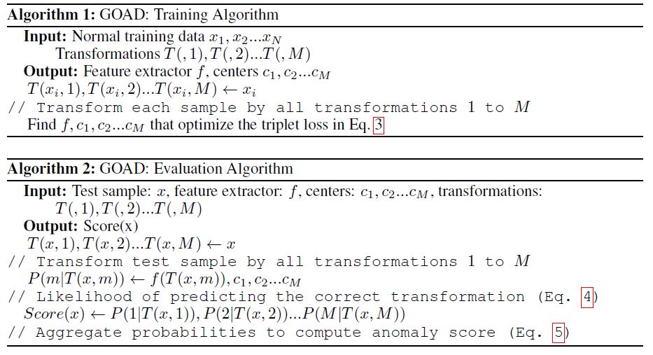
CLASSIFICATION-BASED ANOMALY DETECTION FOR GENERAL DATA
anommaly detection
ICLR 2020 paper
Liron Bergman
Yedid Hoshen
School of Computer Science and Engineering The Hebrew University of Jerusalem, Israel
Classification 기반 Anomaly Detection 연구로는 Deep SVDD 방식과, Geometric-transformation Classification(GEOM) 방식이 대표적임.
다만 기존 연구들은 training set에 포함된 sample에는 잘 동작하나 Generalization 성능은 크게 떨어지는 문제를 가지고 있음.
이를 극복하기 위해 open-set classification 에서 활용되는 idea를 anomaly detection에 접목시키는 연구를 수행하였고, 위에서 소개한 Deep SVDD와 GEOM의 핵심 idea를 합쳐서 일반화 성능을 높인 GOAD 라는 방법론을 제안함.
One-class classification, self-supervised learning, metric learning의 총집합.
1) One-class classification: 정상 데이터만으로 모델을 학습시켜 feature 공간에 투영시키는 사상.
2) Self-supervsied learning: input data에 transformation m을 가하고 어떤 m을 적용했는지 맞추는 self-supervised 모델을 학습한다.
General data에 적용하기 위해 domain knowledge 기반의 transformation이 아닌, 학습되지 않는 random W와 b를 두고 Wx + b를 적용한다.
Adversarial attack에 더 robust한 결과를 보여준다.
3) Metric learning: feature 공간에서 class m에 대한 centroids c를 기준으로 intra-class 간의 거리를 줄이고 inter-class 간의 거리는 벌리는 triplet loss를 계산한다.
- ABSTRACT
- 1 INTRODUCTION
- 2 CLASSIFICATION-BASED ANOMALY DETECTION
- 3 DISTANCE-BASED MULTIPLE TRANSFORMATION CLASSIFICATION
- 4 PARAMETERIZING THE SET OF TRANSFORMATIONS
- 5 EXPERIMENTS
- 6 DISCUSSION
- 7 CONCLUSION
ABSTRACT
Anomaly detection, finding patterns that substantially deviate from those seen previously, is one of the fundamental problems of artificial intelligence.
Recently, classification-based methods were shown to achieve superior results on this task.
In this work, we present a unifying view and propose an open-set method, GOAD, to relax current generalization assumptions.
Furthermore, we extend the applicability of transformation-based methods to non-image data using random affine transformations.
Our method is shown to obtain state-of-the-art accuracy and is applicable to broad data types.
The strong performance of our method is extensively validated on multiple datasets from different domains.
이전에 본 것과 실질적으로 다른 패턴을 찾는, Anomaly detection는 인공지능의 근본적인 문제 중 하나이다.
최근, classification-based methods는 이 작업에서 우수한 결과를 달성하는 것으로 나타났다.
본 연구에서, 우리는 통합 관점을 제시하고 현재의 일반화 가정을 완화하기 위한 open-set method인 GOAD를 제안한다.
또한 random affine transformations을 사용하여 transformation-based methods의 적용 가능성을 non-image data에 확장한다.
우리의 방법은 state-of-the-art accuracy를 얻는 것으로 나타나며 광범위한 데이터 유형에 적용된다.
우리 방법의 강력한 성능은 서로 다른 도메인의 여러 데이터 세트에서 광범위하게 검증된다.
1 INTRODUCTION
Detecting anomalies in perceived data is a key ability for humans and for artificial intelligence.
Humans often detect anomalies to give early indications of danger or to discover unique opportunities.
Anomaly detection systems are being used by artificial intelligence to discover credit card fraud, for detecting cyber intrusion, alert predictive maintenance of industrial equipment and for discovering attractive stock market opportunities.
The typical anomaly detection setting is a one class classification task, where the objective is to classify data as normal or anomalous.
The importance of the task stems from being able to raise an alarm when detecting a different pattern from those seen in the past, therefore triggering further inspection.
This is fundamentally different from supervised learning tasks, in which examples of all data classes are observed.
인식된 데이터에서 Detecting anomalies는 인간과 인공지능의 핵심 능력이다.
인간은 위험의 초기 징후를 제공하거나 고유한 기회를 발견하기 위해 종종 anomalies를 감지한다.
Anomaly detection 시스템은 신용카드 사기 발견, 사이버 침입 탐지, 산업 장비의 경보 예측 유지 및 매력적인 주식 시장 기회 발견을 위해 인공지능에 의해 사용되고 있다.
일반적인 anomaly detection 설정은 단일 분류 작업(one class classification task)이며, 여기서 목적은 데이터를 정상 또는 비정상적으로 분류하는 것이다.
작업의 중요성은 과거에 나타난 패턴과는 다른 패턴을 감지할 때 경보를 발생시킬 수 있기 때문에 추가 검사를 triggering하는 데 있다.
이는 모든 데이터 클래스의 examples를 준수하는 supervised learning tasks와 근본적으로 다르다.
There are different possible scenarios for anomaly detection methods.
In supervised anomaly detection, we are given training examples of normal and anomalous patterns.
This scenario can be quite well specified, however obtaining such supervision may not be possible.
For example in cyber security settings, we will not have supervised examples of new, unknown computer viruses making supervised training difficult.
On the other extreme, fully unsupervised anomaly detection, obtains a stream of data containing normal and anomalous patterns and attempts to detect the anomalous data.
In this work we deal with the semi-supervised scenario.
In this setting, we have a training set of normal examples (which contains no anomalies).
After training the anomaly detector, we detect anomalies in the test data, containing both normal and anomalous examples.
This supervision is easy to obtain in many practical settings and is less difficult than the fully-unsupervised case.
anomaly detection 방법에 대해 여러 가지 가능한 시나리오가 있다.
supervised anomaly detection에서는 정상 및 비정상적인 패턴에 대한 training examples를 제공한다.
이 시나리오는 상당히 잘 명시될 수 있지만, 그러한 supervision을 얻는 것은 불가능할 수 있다.
예를 들어, 사이버 보안 설정에서, 우리는 supervised training을 어렵게 만드는 알려지지 않은 새로운 컴퓨터 바이러스의 supervised examples를 갖고있지는 않을 것이다.
다른 극단적으로, fully unsupervised anomaly detection에서는 정상 및 비정상적인 패턴을 포함하는 데이터 스트림을 얻고 비정상적인 데이터를 탐지하려고 시도한다.
이 작업에서 우리는 semi-supervised 시나리오를 다룬다.
이 설정에서는 anomalies를 포함하지 않는 normal examples의 training set가 있다.
anomaly detector를 training한 후, 우리는 정상 및 비정상적인 예제를 모두 포함하는 test data에서 anomalies를 탐지한다.
이 supervision은 많은 실제 환경에서 얻기 쉽고 fully-unsupervised case보다 덜 어렵다.
Many anomaly detection methods have been proposed over the last few decades.
They can be broadly classified into reconstruction and statistically based methods. Recently, deep learning methods based on classification have achieved superior results.
Most semi-supervised classification-based methods attempt to solve anomaly detection directly, despite only having normal training data.
One example is: Deep-SVDD (Ruff et al., 2018) - one-class classification using a learned deep space.
Another type of classification-based methods is self-supervised i.e. methods that solve one or more classification-based auxiliary tasks on the normal training data, and this is shown to be useful for solving anomaly detection, the task of interest e.g. (Golan & El-Yaniv, 2018).
Self-supervised classification-based methods have been proposed with the object of image anomaly detection, but we show that by generalizing the class of transformations they can apply to all data types.
지난 수십 년 동안 많은 anomaly detection 방법이 제안되었다.
이는 크게 reconstruction과 statistically 방법으로 분류할 수 있다.
최근 classification에 기반한 deep learning 방법이 우수한 결과를 얻었다.
대부분의 semi-supervised classification-based 방법은 정상적인 훈련 데이터만 가지고 있음에도 불구하고 anomaly detection를 직접 해결하려고 시도 한다.
한 가지 예는 다음과 같다: Deep-SVDD (Ruff et al., 2018) - learned deep space를 이용한 one-class classification.
classification-based 방법의 또 다른 유형은 self-supervised 즉, normal training data에 대한 하나 이상의 classification-based auxiliary tasks을 해결하는 방법이며 그것은 연구의 관심 task인, anomaly detection을 해결하는 데 유용한 것으로 나타났다(Golan & El-Yaniv, 2018).
Self-supervised classification-based methods는 image anomaly detection의 object로 제안되었지만, transformations의 class를 일반화함으로써 모든 데이터 유형에 적용할 수 있음을 보여준다.
In this paper, we introduce a novel technique, GOAD, for anomaly detection which unifies current state-of-the-art methods that use normal training data only and are based on classification.
Our method first transforms the data into \(M\) subspaces, and learns a feature space such that inter-class separation is larger than intra-class separation.
For the learned features, the distance from the cluster center is correlated with the likelihood of anomaly.
We use this criterion to determine if a new data point is normal or anomalous.
We also generalize the class of transformation functions to include affine transformation which allows our method to generalize to non-image data.
This is significant as tabular data is probably the most important for applications of anomaly detection.
Our method is evaluated on anomaly detection on image and tabular datasets (cyber security and medical) and is shown to significantly improve over the state-of-the-art.
본 논문에서는 normal training data만 사용하고 classification를 기반으로 하는 현재의 state-of-the-art 방법을 통합하는 anomaly detection을 위한 새로운 기술인 GOAD를 소개한다.
우리의 방법은 먼저 data를 \(M\) subspaces으로 변환하고 inter-class separation이 intra-class separation보다 더 큰 feature space을 학습한다.
학습된 features의 경우, cluster 중심으로부터의 거리는 likelihood of anomaly와 상관 관계가 있다.
이 기준을 사용하여 new data point이 정상인지 비정상인지 여부를 확인한다.
우리는 또한 transformation functions의 class를 일반화하여 우리의 방법을 non-image data로 일반화할 수 있는 affine transformation을 포함한다.
이는 표 형식의 데이터(tabular data)가 anomaly detection의 applications에 가장 중요할 수 있기 때문에 중요하다.
우리의 방법은 image 및 tabular datasets(사이버 보안 및 의료)에 대한 anomaly detection에 대해 평가되며 state-of-the-art보다 크게 개선된 것으로 나타났다.
1.1 PREVIOUS WORKS
Anomaly detection methods can be generally divided into the following categories:
Reconstruction Methods:
Some of the most common anomaly detection methods are reconstruction-based.
The general idea behind such methods is that every normal sample should be reconstructed accurately using a limited set of basis functions, whereas anomalous data should suffer from larger reconstruction costs.
The choice of features, basis and loss functions differentiates between the different methods.
Some of the earliest methods use: nearest neighbors (Eskin et al., 2002), low-rank PCA (Jolliffe, 2011; Candes et al., 2011) or K-means (Hartigan &Wong, 1979) as the reconstruction basis.
Most recently, neural networks were used (Sakurada & Yairi, 2014; Xia et al., 2015) for learning deep basis functions for reconstruction.
Another set of recent methods (Schlegl et al., 2017; Deecke et al., 2018) use GANs to learn a reconstruction basis function.
GANs suffer from mode-collapse and are difficult to invert, which limits the performance of such methods.
Reconstruction Methods:
가장 일반적인 anomaly detection 방법 중 일부는 재구성 기반이다.
이러한 방법의 일반적인 idea는 모든 normal sample은 제한된 기본 함수를 사용하여 정확하게 재구성해야 하는 반면 anomalous data는 더 큰 재구성 비용으로 인해 어려움을 겪어야 한다는 것이다.
features, basis 및 loss functions의 선택은 다른 방법을 구별한다.
가장 초기의 방법으로는 nearest neighbors, low-rank PCA 또는 K-means가 reconstruction basis로 사용된다.
가장 최근에는 reconstruction을 위한 deep basis functions를 학습하기 위해 신경망이 사용되었다.
최근의 또 다른 방법 세트는 reconstruction basis function를 학습하기 위해 GAN을 사용한다.
GAN은 mode-collapse로 어려움을 겪고 invert가 어려우며, 이는 그러한 방법의 성능을 제한한다.
Distributional Methods:
Another set of commonly used methods are distribution-based.
The main theme in such methods is to model the distribution of normal data.
The expectation is that anomalous test data will have low likelihood under the probabilistic model while normal data will have higher likelihoods.
Methods differ in the features used to describe the data and the probabilistic model used to estimate the normal distribution.
Some early methods used Gaussian or Gaussian mixture models.
Such models will only work if the data under the selected feature space satisfies the probabilistic assumptions implicied by the model.
Another set of methods used non-parametric density estimate methods such as kernel density estimate (Parzen, 1962).
Recently, deep learning methods (autoencoders or variational autoencoders) were used to learn deep features which are sometimes easier to model than raw features (Yang et al., 2017).
DAGMM introduced by Zong et al. (2018) learn the probabilistic model jointly with the deep features therefore shaping the features space to better conform with the probabilistic assumption.
Distributional Methods:
일반적으로 사용되는 또 다른 방법 집합은 분포 기반이다.
이러한 방법의 주요 주제는 normal data의 distribution을 model화하는 것이다.
anomalous test data는 probabilistic model에서 low likelihood를 갖는 반면 normal data는 higher likelihood를 가질 것으로 예상된다.
방법은 데이터를 설명하는 데 사용되는 특성과 정규 분포를 추정하는 데 사용되는 확률적 모델에 차이가 있다.
일부 초기 방법은 Gaussian 또는 Gaussian mixture models을 사용했다.
이러한 models은 선택된 feature space의 data가 model에 포함된 확률적 가정을 만족하는 경우에만 작동한다.
또 다른 방법 집합은 커널 밀도 추정(kernel density estimate)과 같은 비모수 밀도 추정(non-parametric density estimate)방법을 사용했다(Parzen, 1962).
최근에는 raw features보다 모델링하기 쉬운 deep features을 학습하기 위해 deep learning 방법(autoencoders 또는 variational autoencoders)이 사용되었다(Yang et al., 2017).
Zong 외 연구진(2018)이 소개한 DAGMM은 probabilistic model jointly with the deep features 학습하여 확률적 가정(probabilistic assumption)을 더 잘 준수하도록 features space을 형성한다.
Classification-Based Methods:
Another paradigm for anomaly detection is separation between space regions containing normal data from all other regions.
An example of such approach is One-Class SVM (Scholkopf et al., 2000), which trains a classifier to perform this separation.
Learning a good feature space for performing such separation is performed both by the classic kernel methods as well as by the recent deep learning approach (Ruff et al., 2018).
One of the main challenges in unsupervised (or semi-supervised) learning is providing an objective for learning features that are relevant to the task of interest.
One method for learning good representations in a self-supervised way is by training a neural network to solve an auxiliary task for which obtaining data is free or at least very inexpensive.
Auxiliary tasks for learning high-quality image features include: video frame prediction (Mathieu et al., 2016), image colorization (Zhang et al., 2016; Larsson et al., 2016), puzzle solving (Noroozi & Favaro, 2016) - predicting the correct order of random permuted image patches.
Recently, Gidaris et al. (2018) used a set of image processing transformations rotation by 0, 90, 180, 270 degrees around the image axis, and predicted the true image orientation has been used to learn high-quality image features.
Golan & El-Yaniv (2018), have used similar image-processing task prediction for detecting anomalies in images.
This method has shown good performance on detecting images from anomalous classes.
In this work, we overcome some of the limitations of previous classification-based methods and extend their applicability of self-supervised methods to general data types.
We also show that our method is more robust to adversarial attacks.
Classification-Based Methods:
anomaly detection의 또 다른 패러다임은 다른 모든 영역의 normal data를 포함하는 공간 영역(space regions) 간의 분리이다.
이러한 접근 방식의 예로는 classifier를 훈련시켜 이러한 분리를 수행하는 One-Class SVM이 있다.
그러한 분리를 수행하기 위한 좋은 feature space를 학습하는 것은 고전적인 kernel methods뿐만 아니라 최근의 deep learning 접근법에 의해 수행된다.
unsupervised (or semi-supervised) learning의 주요 challenges 중 하나는 관심 있는 작업과 관련된 features를 학습하는 목표를 제공하는 것이다.
self-supervised 방식으로 좋은 representations을 학습하는 한 가지 방법은 데이터를 얻는 것이 무료이거나 적어도 매우 저렴한 보조 작업(auxiliary task)을 해결하기 위해 신경망을 훈련시키는 것이다.
고품질 image features을 학습하기 위한 보조 작업(Auxiliary tasks)으로는 video frame prediction, image colorization, puzzle solving이 있다. - random permuted image patches의 올바른 순서를 예측하는 작업이 있다.
최근, Gidaris 외 연구진(2018)은 이미지 축을 중심으로 0도, 90도, 180도, 270도 정도의 image processing transformations rotation 세트를 사용했으며, 실제 이미지 방향이 high-quality image features을 학습하는 데 사용됐다고 예측했다.
Golan & El-Yaniv(2018)는 이미지의 anomalies를 감지하기 위해 유사한 image-processing task prediction을 사용해 왔다.
이 방법은 anomalous classes의 이미지를 감지하는 데 좋은 성능을 보여 주었다.
본 연구에서는 이전 classification-based 방법의 몇 가지 한계를 극복하고 self-supervised 방법의 applicability을 일반 데이터 유형으로 확장하였다.
또한 우리의 방법이 adversarial attacks에 더 강력하다는 것을 보여준다.
2 CLASSIFICATION-BASED ANOMALY DETECTION
Classification-based methods have dominated supervised anomaly detection.
In this section we will analyse semi-supervised classification-based methods:
Let us assume all data lies in space \(R^L\) (where \(L\) is the data dimension).
Normal data lie in subspace \(X \subset R^L\).
We assume that all anomalies lie outside X.
To detect anomalies, we would therefore like to build a classifier \(C\), such that \(C(x) = 1\) if \(x \in X\) and \(C(x) = 0\) if \(x \in R^L / X\).
분류 기반 방법은 supervised anomaly detection을 지배해왔다.
이 section에서는 semi-supervised classification-based methods을 분석한다:
모든 data가 space \(R^L\)(\(L\) : data dimension)에 있다고 가정하자.
Normal data는 subspace \(X \subset R^L\)에 있다.
우리는 모든 anomalies기 X 밖에 있다고 가정한다.
따라서 anomalies을 감지하기 위해 \(x \in X\)이면 \(C(x) = 1\), \(x \in R^L / X\)이면 \(C(x) = 0\)인 classifier \(C\)를 구축하려고 한다.
One-class classification methods attempt to learn \(C\) directly as \(P(x \in X)\).
Classical approaches have learned a classifier either in input space or in a kernel space.
Recently, Deep-SVDD (Ruff et al., 2018) learned end-to-end to
i) transform the data to an isotropic feature space \(f(x)\)
ii) fit the minimal hypersphere of radius \(R\) and center \(c_0\) around the features of the normal training data.
One-class classification methods은 \(C\)를 \(P(x \in X)\)로 직접 학습하려고 시도한다.
고전적인 접근 방식은 input space 또는 kernel space에서 classifier를 학습했다.
최근 Deep-SVDD(Ruff et al., 2018)는
i) data를 isotropic feature space \(f(x)\)로 변환하고
ii) normal training data의 features 주위에 radius \(R\)과 center \(c_0\)의 minimal hypersphere에 맞게 end-to-end로 학습한다.
Test data is classified as anomalous if the following normality score is positive: \(||f(x) - c_0||^2 - R^2\).
Learning an effective feature space is not a simple task, as the trivial solution of \(f(x) = 0 \; \forall x\) results in the smallest hypersphere, various tricks are used to avoid this possibility.
다음 normality score는 positive인 경우 Test data는 anomalous으로 분류된다: \(||f(x) - c_0||^2 - R^2\).
\(f(x) = 0 \; \forall x\)의 trivial solution이 가장 작은 hypersphere에서 발생하므로, 효과적인 feature space 학습은 간단한 task가 아니다, 이러한 가능성을 피하기 위해 다양한 트릭을 사용한다.
Geometric-transformation classification (GEOM), proposed by Golan & El-Yaniv (2018) first transforms the normal data subspace \(X\) into \(M\) subspaces \(X_1 .. X_M\).
This is done by transforming each image \(x \in X\) using \(M\) different geometric transformations (rotation, reflection, translation) into \(T(x,1)..T(x,M)\).
Although these transformations are image specific, we will later extend the class of transformations to all affine transformations making this applicable to non-image data.
They set an auxiliary task of learning a classifier able to predict the transformation label \(m\) given transformed data point \(T(x,m)\).
As the training set consists of normal data only, each sample is \(x \in X\) and the transformed sample is in \(\cup_m X_m\).
The method attempts to estimate the following conditional probability:
\[P(m^{'}|T(x,m)) = \frac{P(T(x,m) \in X_{m^{'}})P(m^{'})}{\sum_{\tilde{m}}P(T(x,m) \in X_{\tilde{m}})P(\tilde{m})} = \frac{P(T(x,m) \in X_{m^{'}})}{\sum_{\tilde{m}}P(T(x,m) \in X_{\tilde{m}})} \qquad (1)\]Geometric-transformation classification (GEOM)는 먼저 normal data subspace \(X\)를 \(M\) subspaces \(X_1 .. X_M\)로 변환한다.
이는 \(M\) different geometric transformations (rotation, reflection, translation)을 사용하여 각 image \(x \in X\)를 \(T(x,1)..T(x,M)\)로 변환함으로써 이루어진다.
이러한 변환은 이미지에 따라 다르긴 하지만 나중에 변환 class를 모든 affine 변환으로 확장하여 non-image data에 적용할 수 있게 할 것이다.
그들은 변환된 data point \(T(x,m)\)가 주어진 transformation label \(m\) 을 예측할 수 있는 classifier를 학습하는 보조 작업을 설정했다.
training set는 normal data로만 구성되므로, 각 sample은 \(x \in X\)이고 변환된 sample은 \(\cup_m X_m\)이다.
이 방법은 다음과 같은 조건부 확률(conditional probability)을 추정하려고 한다.
,Where the second equality follows by design of the training set, and where every training sample is transformed exactly once by each transformation leading to equal priors.
For anomalous data \(x \in R^L \backslash X\), by construction of the subspace, if the transformations \(T\) are one-to-one, it follows that the transformed sample does not fall in the appropriate subspace: \(T(x,m) \in R^L \backslash X_m\).
anomalous data \(x \in R^L \backslash X\)에서, subspace의 construction에 의해, transformations \(T\)가 one-to-one이면, transformed sample이 적절한 subspace인 \(T(x,m) \in R^L \backslash X_m\)에 속하지 않는다.
GEOM uses \(P(m\|T(x,m))\) as a score for determining if \(x\) is anomalous i.e. that \(x \in R^L \backslash X\).
GEOM gives samples with low probabilities \(P(m\|T(x,m))\) high anomaly scores.
GEOM은 \(x\)가 anomalous인지, 즉 \(x \in R^L \backslash X\)인지를 결정하기 위한 score로 \(P(m\|T(x,m))\)를 사용한다.
GEOM은 낮은 probabilities \(P(m\|T(x,m))\) 높은 anomaly scores를 가진 samples을 제공한다.
A significant issue with this methodology, is that the learned classifier \(P(m^{'}|T(x,m))\) is only valid for samples \(x \in X\) which were found in the training set.
For \(x \in R^L\backslash X\) we should in fact have \(P(T(x,m) \in X_{m^{'}} ) = 0\) for all \(m = 1..M\) (as the transformed \(x\) is not in any of the subsets).
This makes the anomaly score \(P(m^{'}|T(x,m))\) have very high variance for anomalies.
이 방법론의 중요한 문제는 학습된 classifier \(P(m^{'}|T(x,m))\)가 training set에서 발견된 samples \(x \in X\)에만 valid하다는 것이다.
\(x \in R^L\backslash X\)에서, 우리는 사실 모든 \(m = 1..M\)에 대해 \(P(T(x,m) \in X_{m^{'}}) = 0\)를 가져야 한다.(transformed \(x\)가 subsets에 있지 않기 때문에)
이로 인해 anomaly score \(P(m^{'}|T(x,m))\)는 anomalies에 대한 변동이 매우 높다.
One way to overcome this issue is by using examples of anomalies \(x_a\) and training \(P(m|T(x,m)) = 1/M\) on anomalous data.
This corresponds to the supervised scenario and was recently introduced as Outlier Exposure (Hendrycks et al., 2018).
Although getting such supervision is possible for some image tasks (where large external datasets can be used) this is not possible in the general case e.g. for tabular data which exhibits much more variation between datasets.
이 문제를 해결하는 한 가지 방법은 anomalies \(x_a\)의 examples를 사용하고 anomalous data에 대해 \(P(m|T(x,m)) = 1/M\)를 training시키는 것이다.
이는 supervised scenario에 해당하며 최근 Outlier Exposure(Hendrycks et al., 2018)로 소개되었다.
일부 image tasks(large external datasets를 사용할 수 있는 경우)에서는 이러한 supervision을 받을 수 있지만, 일반적인 경우(예: datasets 간에 훨씬 더 많은 변동(variation)을 보이는 tabular data)에서는 가능하지 않다.
3 DISTANCE-BASED MULTIPLE TRANSFORMATION CLASSIFICATION
We propose a novel method to overcome the generalization issues highlighted in the previous section by using ideas from open-set classification (Bendale & Boult, 2016).
Our approach unifies one-class and transformation-based classification methods.
Similarly to GEOM, we transform \(X\) to \(X_1..X_M\).
We learn a feature extractor \(f(x)\) using a neural network, which maps the original input data into a feature representation.
Similarly to deep OC methods, we model each subspace \(X_m\) mapped to the feature space \({f(x)|x \in X_m}\) as a sphere with center \(c_m\).
The probability of data point \(x\) after transformation \(m\) is parameterized by \(P(T(x,m) \in X^{'}_m ) = \frac{1}{Z} e^{-(f(T(x,m))-c^{'}_m)^2}\).
우리는 open-set classification의 아이디어를 사용하여 이전 section에서 강조된 generalization 문제를 극복하기 위한 새로운 방법을 제안한다(Bendale & Boult, 2016).
우리의 접근 방식은 one-class와 transformation-based classification methods을 통합한다.
GEOM과 유사하게, 우리는 \(X\)를 \(X_1..X_M\)로 변환한다.
우리는 신경망(neural network)을 사용하여 feature extractor \(f(x)\)를 학습하며, 이는 original input data를 feature representation으로 매핑한다.
deep OC methods와 유사하게, 우리는 feature space \({f(x)|x \in X_m}\)에 매핑된 각 subspace \(X_m\)을 center \(c_m\)을 가진 sphere로 모델링한다.
transformation \(m\)이 \(P(T(x,m) \in X^{'}_m ) = \frac{1}{Z} e^{-(f(T(x,m))-c^{'}_m)^2}\)로 매개 변수화된 후 data point \(x\)의 probability이다.
The classifier predicting transformation \(m\) given a transformed point is therefore: \[P(m^{'}|T(x,m)) = \frac{e^{-||f(T(x,m))-c_{m^{'}}||^2}}{\sum_{\tilde{m}}e^{-||f(T(x,m))-c_{\tilde{m}}||^2}} \qquad (2)\]
The centers \(c_m\) are given by the average feature over the training set for every transformation i.e. \(c_m = \frac{1}{N} \sum_{x \in X}f(T(x,m))\).
One option is to directly learn f by optimizing cross-entropy between \(P(m^{'}|T(x,m))\) and the correct label on the normal training set.
In practice we obtained better results by training \(f\) using the center triplet loss (He et al., 2018), which learns supervised clusters with low intra-class variation, and high-inter-class variation by optimizing the following loss function (where \(s\) is a margin regularizing the distance between clusters):
\[L=\sum_{i} \max (||f(T(x_i,m))) - c_m||^2 + s - \min_{\tilde{m} \ne m}||f(T(x_i,m))-c_{m^{'}}||^2,0) \qquad (3)\]centers \(c_m\)은 모든 transformation에 대한 training set에 대한 average feature에 의해 주어진다.
즉, \(c_m = \frac{1}{N} \sum_{x \in X}f(T(x,m))\).
한 가지 옵션은 \(P(m^{'}|T(x,m))\)와 normal training set의 올바른 label 사이의 cross-entropy를 optimizing하여 \(f\)를 직접 학습하는 것이다.
실제로 우리는 클래스 내 변동이 낮은 중앙 삼중 손실(He et al., 2018)과 다음 loss function(여기서 \(s\)는 clusters 간 거리를 정규화하는 margin)을 최적화하여 high-inter-class variation와 low intra-class variation로 supervised clusters를 학습하는 center triplet loss (He et al., 2018)을 사용하여 \(f\)를 training 함으로써 더 나은 결과를 얻었다:
Having learned a feature space in which the different transformation subspaces are well separated, we use the probability in Eq. 2 as a normality score.
However, for data far away from the normal distributions, the distances from the means will be large.
A small difference in distance will make the classifier unreasonably certain of a particular transformation.
To add a general prior for uncertainty far from the training set, we add a small regularizing constant \(\epsilon\) to the probability of each transformation.
This ensures equal probabilities for uncertain regions:
\[\tilde{P(m^{'}|T(x,m))} = \frac{e^{-||f(T(x,m))-c_{m^{'}}||^2 + \epsilon}}{\sum_{\tilde{m}}e^{-||f(T(x,m))-c_{\tilde{m}}||^2} + M \cdot \epsilon} \qquad (4)\]서로 다른 transformation subspaces가 잘 분리되는 feature space를 학습하여 Eq. 2의 probability을 normality score로 사용한다.
그러나 normal distributions에서 멀리 떨어진 data의 경우 평균으로부터의 거리가 크다.
거리에 작은 차이가 있으면 classifier가 특정 변환을 불합리하게 확신하게 된다.
training set에서 멀리 떨어진 uncertainty에 대한 general prior을 추가하기 위해, 우리는 각 변환 확률에 작은 정규화 상수 \(\epsilon\)을 추가한다.
이렇게 하면 불확실한 영역에 대해 동일한 확률이 보장된다.
At test time we transform each sample by the \(M\) transformations.
By assuming independence between transformations, the probability that \(x\) is normal (i.e. \(x \in X\)) is the product of the probabilities that all transformed samples are in their respective subspace.
For log-probabilities the total score is given by:
\[Score(x) = -\log P(x \in X) = -\sum_m \log \tilde{P}(T(x,m) \in X_m) = -\sum_m \log \tilde{P}(m|T(x,m)) \qquad (5)\]test time에 우리는 \(M\) transformations을 통해 각 sample을 transform한다.
transformations 간의 independence을 가정함으로써, \(x\)가 정규일 확률(즉, \(x \in X\))은 변환된 모든 samples이 respective subspace에 있을 확률의 product이다.
log-probabilities의 경우 total score는 다음과 같다.
The score computes the degree of anomaly of each sample.
Higher scores indicate a more anomalous sample.
4 PARAMETERIZING THE SET OF TRANSFORMATIONS
Geometric transformations have been used previously for unsupervised feature learning by Gidaris et al. (2018) as well as by GEOM (Golan & El-Yaniv, 2018) for classification-based anomaly detection.
This set of transformations is hand-crafted to work well with convolutional neural networks (CNNs) which greatly benefit from preserving neighborhood between pixels.
This is however not a requirement for fully-connected networks.
Anomaly detection often deals with non-image datasets e.g. tabular data.
Tabular data is very commonly used on the internet e.g. for cyber security or online advertising.
Such data consists of both discrete and continuous attributes with no particular neighborhoods or order.
The data is one-dimensional and rotations do not naturally generalize to it.
To allow transformation-based methods to work on general data types, we therefore need to extend the class of transformations.
Geometric transformations은 이전에 classification-based anomaly detection을 위해 GEOM(Golan & El-Yaniv, 2018)뿐만 아니라 Gidaris et al. (2018)에 의해 unsupervised feature learning에 사용되어왔다.
이러한 변환 세트는 pixels 간 neighborhood을 보존하는 데 큰 benefit을 갖는 CNN(Convolutional Neural Network)과 잘 작동하도록 수작업으로 제작되었다.
그러나 fully-connected networks의 requirement는 아니다.
Anomaly detection는 종종 non-image datasets(예: tabular data)를 다룬다.
Tabular data는 사이버 보안이나 온라인 광고와 같은 인터넷 상에서 매우 흔하게 사용된다.
이러한 데이터는 특별한 neighborhoods나 순서가 없는 이산형(discrete) 및 연속형(continuous) 속성(attributes)으로 구성된다.
데이터는 1차원이며 회전은 자연스럽게 일반화되지 않는다.
따라서 transformation-based methods이 일반적인 data types에 대해 작동하도록 하려면 transformations class를 확장해야 한다.
We propose to generalize the set of transformations to the class of affine transformations (where we have a total of \(M\) transformations):
\[T(x,m) = W_{m}x + b_m \qquad \qquad (6)\]우리는 affine 변환(총 \(M\) transformations이 있는 경우) class로 변환 세트를 일반화할 것을 제안한다:
It is easy to verify that all geometric transformations in Golan & El-Yaniv (2018) (rotation by a multiple of 90 degrees, flips and translations) are a special case of this class (x in this case is the set of image pixels written as a vector).
The affine class is however much more general than mere permutations, and allows for dimensionality reduction, non-distance preservation and random transformation by sampling \(W,b\) from a random distribution.
Golan & El-Yaniv(2018)의 모든 geometric transformations(90도 배수로 회전, flips과 translations)이 이 class의 special case임을 쉽게 확인할 수 있다(이 경우 x는 벡터로 작성된 이미지 픽셀 집합이다).
그러나 affine class는 단순한 순열보다 훨씬 일반적이며, random distribution에서 \(W, b\)를 샘플링하여 차원 축소, 비거리 보존 및 무작위 변환을 허용한다.
Apart from reduced variance across different dataset types where no a priori knowledge on the correct transformation classes exists, random transformations are important for avoiding adversarial examples.
Assume an adversary wishes to change the label of a particular sample from anomalous to normal or vice versa.
This is the same as requiring that \(\tilde{P} (m^{'}\|T(x,m))\) has low or high probability for \(m^{'} = m\).
If \(T\) is chosen deterministically, the adversary may create adversarial examples against the known class of transformations (even if the exact network parameters are unknown).
Conversely, if \(T\) is unknown, the adversary must create adversarial examples that generalize across different transformations, which reduces the effectiveness of the attack.
올바른 변환 클래스에 대한 사전 지식이 없는 서로 다른 dataset 유형에 대한 분산 감소 외에도, random transformations은 adversarial examples를 피하는 데 중요하다.
adversary가 특정 sample의 label을 anomalous에서 normal 또는 그 반대로 변경하기를 원한다고 가정한다.
이는 \(\tilde{P} (m^{'}\|T(x,m))\)가 \(m^{'} = m\)에 대해 낮은 확률 또는 높은 확률을 요구하는 것과 같다.
\(T\)를 결정적으로 선택하는 경우, adversary는 알려진 변환 class에 대한 adversarial examples를 생성할 수 있다(정확한 network parameters를 알 수 없는 경우에도).
반대로 \(T\)를 알 수 없는 경우, adversary는 서로 다른 변환에 걸쳐 일반화하는 adversarial examples를 만들어야 하므로 공격의 효과가 감소한다.
To summarize, generalizing the set of transformations to the affine class allows us to: generalize to non-image data, use an unlimited number of transformations and choose transformations randomly which reduces variance and defends against adversarial examples.
요약하면, affine class로 변환 집합을 일반화하면 다음과 같이 non-image data로 일반화하고, 무제한 변환을 사용하고, 분산을 줄이고 adversarial examples에 대해 방어하는 변환을 무작위로 선택할 수 있다.
5 EXPERIMENTS
We perform experiments to validate the effectiveness of our distance-based approach and the performance of the general class of transformations we introduced for non-image data.
우리는 non-image data에 대해 소개한 distance-based approach의 효과와 general class of transformations의 성능을 검증하기 위한 실험을 수행한다.
5.1 IMAGE EXPERIMENTS
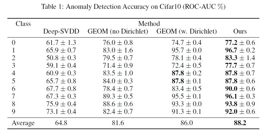
Cifar10: To evaluate the performance of our method, we perform experiments on the Cifar10 dataset.
We use the same architecture and parameter choices of Golan & El-Yaniv (2018), with our distance-based approach.
We use the standard protocol of training on all training images of a single digit and testing on all test images.
Results are reported in terms of AUC.
In our method, we used a margin of \(s = 0.1\) (we also run GOAD with \(s = 1\), shown in the appendix).
Similarly to He et al. (2018), to stabilize training, we added a softmax + cross entropy loss, as well as \(L_2\) norm regularization for the extracted features \(f(x)\).
We compare our method with the deep one-class method of Ruff et al. (2018) as well as Golan & El-Yaniv (2018) without and with Dirichlet weighting.
We believe the correct comparison is without Dirichlet post-processing, as we also do not use it in our method.
Our distance based approach outperforms the SOTA approach by Golan & El-Yaniv (2018), both with and without Dirichlet (which seems to improve performance on a few classes).
This gives evidence for the importance of considering the generalization behavior outside the normal region used in training.
Note that we used the same geometric transformations as Golan & El-Yaniv (2018).
Random affine matrices did not perform competitively as they are not pixel order preserving, this information is effectively used by CNNs and removing this information hurts performance.
This is a special property of CNN architectures and image/time series data.
As a rule of thumb, fully-connected networks are not pixel order preserving and can fully utilize random affine matrices.
Cifar10: 방법의 성능을 평가하기 위해 Cifar10 dataset에 대한 실험을 수행한다.
우리는 distance-based 접근법과 함께 Golan & El-Yaniv (2018)의 동일한 아키텍처(GEOM)와 parameter를 선택한다.
우리는 한 자릿수의 모든 training images에 대한 training과 모든 test images에 대한 testing의 standard protocol을 사용한다.
결과는 AUC로 보고된다.
우리의 방법에서는 \(s = 0.1\)의 margin을 사용했다(부록에 표시된 \(s = 1\)로 GOAD를 실행하기도 한다).
He et al.(2018)와 유사하게, 우리는 training을 안정화하기 위해 추출된 features \(f(x)\)에 대해 \(L_2\) norm regularization와 함께 softmax + cross entropy loss를 추가했다.
우리는 우리의 방법을 Dirichlet 가중치를 사용하고 사용하지 않고 Golan & El-Yaniv(2018)뿐만 아니라 Ruff et al.(2018)의 deep one-class method와 비교한다.
우리는 Dirichlet 후처리가 없는 정확한 비교가 가능하다고 믿는다. 왜냐하면 우리는 또한 Dirichlet을 우리의 방법에도 사용하지 않기 때문이다.
우리의 distance-based 접근 방식은 (일부 클래스에서 성능을 향상시키는 것으로 보이는)Dirichlet가 있는것과 없는거 모두, Golan & El-Yaniv(2018)의 SOTA 접근 방식을 능가한다.
이는 training에 사용되는 normal region 밖의 일반화를 고려하는 것의 중요성을 보여주는 증거를 제공한다.
Golan & El-Yaniv(2018)와 동일한 geometric transformations을 사용했다는 점에 유의한다.
무작위 affine 행렬은 pixel 순서가 보존되지 않기 때문에 경쟁적으로 수행되지 않았으며, 이 정보는 CNN에 의해 효과적으로 사용되며 이 정보를 제거하면 성능이 저하된다.
이것은 CNN 아키텍처와 image/time series data의 특수한 속성이다.
원칙적으로, fully-connected networks는 pixel 순서를 보존하지 않으며 무작위 affine 행렬을 완전히 활용할 수 있다.
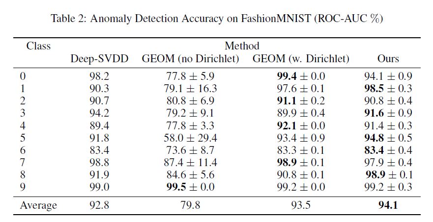
FasionMNIST: In Tab. 2, we present a comparison between our method (GOAD) and the strongest baseline methods (Deep SVDD and GEOM) on the FashionMNIST dataset.
We used exactly the same setting as Golan & El-Yaniv (2018).
GOAD was run with s = 1. OCSVM and GEOM with Dirichlet were copied from their paper.
We run their method without Dirichlet and presented it in the table (we verified the implementation by running their code with Dirichlet and replicated the numbers in the paper).
It appears that GEOM is quite dependent on Dirichlet for this dataset, whereas we do not use it at all.
GOAD outperforms all the baseline methods.
FasionMNIST: Tab. 2에서 우리는 FashionMNIST dataset에서 우리의 method(GOAD)와 strongest baseline methods(Deep SVDD and GEOM)을 비교한다.
Golan & El-Yaniv(2018)와 정확히 동일한 설정을 했다.
GOAD는 s= 1. OCSVM and GEOM with Dirichlet는 그들의 논문에서 복사해왔다.
우리는 Dirichlet 없이 그들의 방법을 실행하고 표에 제시하였다(Dirichlet으로 코드를 실행하여 구현을 검증하고 논문의 숫자를 복제했다).
GEOM은 dataset에 대해 Dirichlet에 상당히 의존하는 반면, 우리는 전혀 사용하지 않았다.
GOAD는 모든 기본 방법을 능가한다.
Adversarial Robustness: Let us assume an attack model where the attacker knows the architecture and the normal training data and is trying to minimally modify anomalies to look normal.
We examine the merits of two settings
i) the adversary knows the transformations used (non-random)
ii) the adversary uses another set of transformations.
To measure the benefit of the randomized transformations, we train three networks A, B, C.
Networks A and B use exactly the same transformations but random parameter initialization prior to training.
Network C is trained using other randomly selected transformations.
The adversary creates adversarial examples using PGD (Madry et al., 2017) based on network A (making anomalies appear like normal data).
On Cifar10, we randomly selected 8 transformations from the full set of 72 for A and B, another randomly selected 8 transformations are used for C.
We measure the increase of false classification rate on the adversarial examples using the three networks.
The average increase in performance of classifying transformation correctly on anomalies (causing lower anomaly scores) on the original network A was 12.8%, the transfer performance for B causes an increase by 5.0% on network B which shared the same set of transformation, and 3% on network C that used other rotations.
This shows the benefits of using random transformations.
Adversarial Robustness: attacker가 아키텍처와 normal training data를 알고 anomalies를 최소한으로 수정하여 normal로 보이도록 하는 공격 모델을 가정하자.
우리는 두 가지 설정의 장점을 조사한다.
i) adversary가 사용된 변환을 알고 있다(non-random).
ii) adversary는 다른 변환 집합을 사용한다.
무작위 변환의 이점을 측정하기 위해, 우리는 세 개의 networks A, B, C를 훈련시킨다.
Networks A와 B는 training 전에 정확히 동일한 변환을 사용하지만 random parameter initialization를 사용한다.
Network C는 other randomly selected transformations을 사용하여 train된다.
adversary는 Network A(anomalies를 normal data와 같이 표시)에 기반한 PGD(Madry et al., 2017)를 사용하여 adversarial examples를 생성한다.
Cifar10에서는 A와 B에 대한 72개의 전체 집합에서 8개의 변환을 무작위로 선택했으며, 다른 8개의 변환은 C에 사용된다.
우리는 세 개의 networks를 사용하여 adversarial examples에서 false classification rate의 증가를 측정한다.
original network A에서 anomalies(anomaly scores가 낮아짐)에서 변환을 올바르게 분류하는 평균 성능 증가는 12.8%, B에 대한 transfer performance는 동일한 변환 세트를 공유하는 network B에서 5.0%, other rotations을 사용한 network C에서 3%의 증가를 유발했다.
이것은 random transformations을 사용할 때의 이점을 보여준다.
5.2 TABULAR DATA EXPERIMENTS
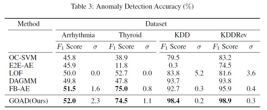
Datasets: We evaluate on small-scale medical datasets Arrhythmia, Thyroid as well as large-scale cyber intrusion detection datasets KDD and KDDRev.
Our configuration follows that of Zong et al. (2018).
Categorical attributes are encoded as one-hot vectors.
For completeness the datasets are described in the appendix A.2. We train all compared methods on 50% of the normal data.
The methods are evaluated on 50% of the normal data as well as all the anomalies.
Datasets: 소규모 의료 데이터 세트 부정맥, 갑상선뿐만 아니라 대규모 사이버 침입 탐지 데이터 세트 KDD 및 KDDRev에 대해 평가한다.
우리의 구성은 Zong 등(2018)과 같다.
범주형 특성은 원핫 벡터로 인코딩됩니다.
완전성을 위해 데이터 세트는 부록 A.2에 설명되어 있다. 우리는 모든 비교 방법을 정규 데이터의 50%에 대해 훈련한다.
이 방법은 정규 데이터의 50%와 모든 이상 징후에서 평가됩니다.
Baseline methods: The baseline methods evaluated are: One-Class SVM (OC-SVM, Scholkopf et al. (2000)), End-to-End Autoencoder (E2E-AE), Local Outlier Factor (LOF, Breunig et al. (2000)).
We also evaluated deep distributional method DAGMM (Zong et al., 2018), choosing their strongest variant.
To compare against ensemble methods e.g. Chen et al. (2017), we implemented the Feature Bagging Autoencoder (FB-AE) with autoencoders as the base classifier, feature bagging as the source of randomization, and average reconstruction error as the anomaly score.
OC-SVM, E2E-AE and DAGMM results are directly taken from those reported by Zong et al. (2018). LOF and FB-AE were computed by us.
Baseline methods: 평가된 기준 방법은 One-Class SVM(OC-SVM, Scholkopf 등)이다. (2000), 단대단 자동 인코더(E2E-AE), 국소 특이치 인자(LOF, Breunig 등) (2000)).
또한 심층 분포 방법 DAGMM(종 등, 2018)을 평가하여 가장 강력한 변형을 선택했다.
예를 들어 앙상블 방법과 비교한다. Chen 외 연구진(2017)은 자동 인코더를 기본 분류기로, 기능 백킹을 무작위화의 소스로, 평균 재구성 오류를 이상 점수로 구현했다.
OC-SVM, E2E-AE 및 DAGMM 결과는 Zong 등(2018)이 보고한 결과에서 직접 가져온 것이다. LOF와 FB-AE는 우리가 계산했다.
Implementation of GOAD: We randomly sampled transformation matrices using the normal distribution for each element.
Each matrix has dimensionality \(L \times r\), where L is the data dimension and r is a reduced dimension.
For Arryhthmia and Thyroid we used r = 32, for KDD and KDDrev we used r = 128 and r = 64 respectively, the latter due to high memory requirements.
We used 256 tasks for all datasets apart from KDD (64) due to high memory requirements.
We set the bias term to 0.
For C we used fully-connected hidden layers and leaky-ReLU activations (8 hidden nodes for the small datasets, 128 and 32 for KDDRev and KDD).
We optimized using ADAM with a learning rate of 0.001.
Similarly to He et al. (2018), to stabilize the triplet center loss training, we added a softmax + cross entropy loss.
We repeated the large-scale experiments 5 times, and the small scale GOAD experiments 500 times (due to the high variance).
We report the mean and standard deviation (\(\sigma\)).
Following the protocol in Zong et al. (2018), the decision threshold value is chosen to result in the correct number of anomalies e.g. if the test set contains \(N_a\) anomalies, the threshold is selected so that the highest Na scoring examples are classified as anomalies.
True positives and negatives are evaluated in the usual way.
Some experiments copied from other papers did not measure standard variation and we kept the relevant cell blank.
Implementation of GOAD: 각 원소에 대한 정규 분포를 사용하여 변환 행렬을 랜덤하게 샘플링했습니다.
각 행렬에는 치수 L이 있으며, 여기서 L은 데이터 치수이고 r은 축소 치수이다.
Arrythmia와 갑상선의 경우 r = 32를, KDDR 및 KDDrev의 경우 r = 128과 r = 64를 각각 사용했는데, 이는 메모리 요구량이 높기 때문이다.
높은 메모리 요구 사항으로 인해 KDD(64)를 제외한 모든 데이터 세트에 256개의 작업을 사용했다.
bias term을 0으로 설정합니다.
C의 경우 fully-connected hidden layers와 leaky-ReLU activations를 사용했습니다.(8 hidden nodes for the small datasets, 128 and 32 for KDDRev and KDD) 우리는 학습률이 0.001인 ADAM을 사용하여 최적화했다.
He et al. (2018)와 유사하게, 트리플트 센터 손실 훈련을 안정화시키기 위해 소프트맥스 + 크로스 엔트로피 손실을 추가했다.
대규모 실험은 5회 반복했고, 소규모 GOAD 실험은 500회 반복했다(높은 분산 때문에).
평균 및 표준 편차($\sigma\()를 보고한다. Zong et al. (2018)의 protocol에 이어, 결정 임계값을 선택하여 테스트 세트에\)N_a$$ anomalies이 포함된 경우, 가장 높은 Na 점수 매기기 예제를 이상 징후로 분류할 수 있도록 올바른 이상 징후 수를 산출한다.
진정한 긍정과 부정은 일반적인 방법으로 평가됩니다.
다른 논문에서 복사한 일부 실험은 표준 변동을 측정하지 않았으며 관련 셀을 공백으로 유지했습니다.
Results
Arrhythmia: The Arrhythmia dataset was the smallest examined.
A quantitative comparison on this dataset can be seen in Tab. 3.
OC-SVM and DAGMM performed reasonably well.
Our method is comparable to FB-AE.
A linear classifier \(C\) performed better than deeper networks (which suffered from overfitting).
Early stopping after a single epoch generated the best results.
부정맥: 부정맥 데이터 세트가 가장 적게 검사되었다.
이 데이터 세트에 대한 정량적 비교는 표 3에서 확인할 수 있다.
OC-SVM과 DAGMM은 상당히 잘 수행되었다.
우리의 방법은 FB-AE에 필적한다.
linear classifier \(C\)는 (과적합을 겪는)deeper networks보다 더 잘 수행되었다.
single epoch후 Early stopping는 것이 최상의 결과를 낳았다.
Thyroid: Thyroid is a small dataset, with a low anomaly to normal ratio and low feature dimensionality.
A quantitative comparison on this dataset can be seen in Tab. 3.
Most baselines performed about equally well, probably due to the low dimensionality.
On this dataset, we also found that early stopping after a single epoch gave the best results.
The best results on this dataset, were obtained with a linear classifier.
Our method is comparable to FB-AE and beat all other baselines by a wide margin.
갑상선: 갑상선은 정규 비율에 대한 이상 징후와 기능 치수가 낮은 작은 데이터 세트이다.
이 데이터 세트에 대한 정량적 비교는 표 3에서 확인할 수 있다.
대부분의 기준선은 낮은 차원성 때문에 거의 똑같이 잘 수행되었다.
이 데이터 세트에서도 단일 시대 이후 조기 중단이 최상의 결과를 제공한다는 것을 발견했다.
이 데이터 세트에 대한 최상의 결과는 선형 분류기로 얻어졌다.
우리의 방법은 FB-AE와 비슷하며 다른 모든 기준선을 큰 폭으로 능가한다.
KDDCUP99: The UCI KDD 10% dataset is the largest dataset examined.
A quantitative comparison on this dataset can be seen in Tab. 3.
The strongest baselines are FB-AE and DAGMM.
Our method significantly outperformed all baselines.
We found that large datasets have different dynamics from very small datasets.
On this dataset, deep networks performed the best.
We also, did not need early stopping.
The results are reported after 25 epochs.
KDDCUP99:자전거 경기 미국의 10%의 데이터 가장 큰 데이터 조사하였습니다.
이 데이터 집합에 관한 양적 비교 탭. 3에서 볼 수 있다.
가장 강한 베이스 라인 있FB-AE과 DAGMM.
우리의 메서드는 모든 베이스 라인.
우리는 큰 데이터 집합은 매우 작은 데이터 집합에서 다른 역학을 가지고 있다고 한다.
이 데이터 집합에, 깊은 네트워크 최고를 수행했다.
우리는 또한, 일찍 제동이 필요하지 않았다.
그 결과는 25시대 이후 보고되고 있다.
KDD-Rev: The KDD-Rev dataset is a large dataset, but smaller than KDDCUP99 dataset.
A quantitative comparison on this dataset can be seen in Tab. 3.
Similarly to KDDCUP99, the best baselines are FB-AE and DAGMM, where FB-AE significantly outperforms DAGMM.
Our method significantly outperformed all baselines.
Due to the size of the dataset, we did not need early stopping.
The results are reported after 25 epochs.
KDD-Rev: KDD-Rev 데이터 세트는 큰 데이터 세트이지만 KDDCUP99 데이터 세트보다 작습니다.
이 데이터 세트에 대한 정량적 비교는 표 3에서 확인할 수 있다.
KDDCUP99와 유사하게, 최고의 기준선은 FB-AE와 DAGMM이며, 여기서 FB-AE는 DAGMM을 크게 능가한다.
우리의 방법은 모든 기준치를 크게 앞질렀다.
데이터 세트의 크기 때문에, 우리는 일찍 중지할 필요가 없었다.
결과는 25시 이후에 보고된다.
Adversarial Robustness: Due to the large number of transformations and relatively small networks, adversarial examples are less of a problem for tabular data.
PGD generally failed to obtain adversarial examples on these datasets.
On KDD, transformation classification accuracy on anomalies was increased by 3.7% for the network the adversarial examples were trained on, 1.3% when transferring to the network with the same transformation and only 0.2% on the network with other randomly selected transformations.
This again shows increased adversarial robustness due to random transformations.
적대적 견고성: 변환의 수가 많고 네트워크가 상대적으로 작기 때문에, 적대적 예는 표 형식의 데이터에 대한 문제가 덜하다.
PGD는 일반적으로 이러한 데이터 세트에 대한 적대적 예를 얻지 못했다.
KDD에서는, 이상 징후들에 대한 변환 분류 정확도가 적대적인 예들이 훈련된 네트워크에 대해 3.7% 증가했고, 동일한 변환으로 네트워크로 전송할 때는 1.3%, 무작위로 선택된 다른 변환이 있는 네트워크에서 0.2% 증가했다.
이는 무작위 변환으로 인한 적대적 견고성의 증가를 다시 보여준다.
Further Analysis
Contaminated Data: This paper deals with the semi-supervised scenario i.e. when the training dataset contains only normal data.
In some scenarios, such data might not be available but instead we might have a training dataset that contains a small percentage of anomalies.
To evaluate the robustness of our method to this unsupervised scenario, we analysed the KDDCUP99 dataset, when X% of the training data is anomalous.
To prepare the data, we used the same normal training data as before and added further anomalous examples.
The test data consists of the same proportions as before.
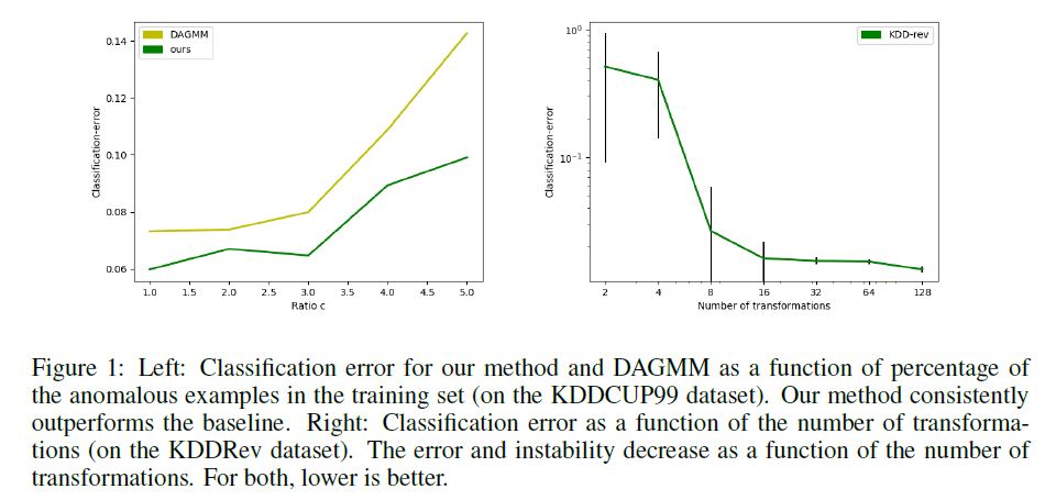
The results are shown in Fig. 1. Our method significantly outperforms DAGMM for all impurity values, and degrades more graceful than the baseline.
This attests to the effectiveness of our approach.
Results for the other datasets are presented in Fig. 3, showing similar robustness to contamination.
오염된 데이터: 본 논문은 훈련 데이터 세트에 정규 데이터만 포함된 반지도 시나리오를 다룬다.
일부 시나리오에서는 이러한 데이터를 사용할 수 없을 수 있지만 대신 약간의 이상 징후를 포함하는 교육 데이터 세트가 있을 수 있다.
이 비지도 시나리오에 대한 우리의 방법의 견고성을 평가하기 위해, 우리는 훈련 데이터의 X%가 비정상적일 때 KDDCUP99 데이터 세트를 분석하였다.
데이터를 준비하기 위해 이전과 동일한 정규 교육 데이터를 사용하고 비정상적인 예를 추가했습니다.
검정 데이터는 이전과 동일한 비율로 구성됩니다.
결과는 그림 1에 나와 있습니다. 우리의 방법은 모든 불순도 값에 대해 DAGMM을 크게 능가하며 기준값보다 더 우아하게 저하된다.
이것은 우리의 접근법의 효과를 입증한다.
다른 데이터 세트에 대한 결과는 그림 3에 제시되어 오염과 유사한 견고성을 보여준다.
Number of Tasks: One of the advantages of GOAD, is the ability to generate any number of tasks.
We present the anomaly detection performance on the KDD-Rev dataset with different numbers of tasks in Fig. 1.
We note that a small number of tasks (less than 16) leads to poor results.
From 16 tasks, the accuracy remains stable.
We found that on the smaller datasets (Thyroid, Arrhythmia) using a larger number of transformations continued to reduce \(F_1\) score variance between differently initialized runs (Fig. 2).
작업 수: GOAD의 장점 중 하나는 여러 작업을 생성할 수 있다는 것입니다.
우리는 KDD-Rev 데이터 세트에 대한 이상 탐지 성능을 그림 1에서 서로 다른 수의 작업으로 제시한다.
우리는 적은 수의 작업(16개 미만)이 좋지 않은 결과를 초래한다는 점에 주목한다.
16개 과제에서 정확도는 안정적으로 유지됩니다.
우리는 더 많은 변환을 사용하는 소규모 데이터 세트(thyroid, 부정맥)에서 서로 다른 초기화 실행 간의 $F_1$ 점수 차이를 계속 줄인다는 것을 발견했다(그림 2).
6 DISCUSSION
Openset vs. Softmax: The openset-based classification presented by GOAD resulted in performance improvement over the closed-set softmax approach on Cifar10 and FasionMNIST.
In our experiments, it has also improved performance in KDDRev. Arrhythmia and Thyroid were comparable.
As a negative result, performance of softmax was better on KDD (F1 = 0.99).
Openset vs. Softmax : GOAD가 제시한 openset-based classification는 Cifar10 및 FasionMNIST에서 closed-set softmax approach에 비해 성능 향상을 가져왔다.
우리의 실험에서, 그것은 또한 KDDRev의 성능을 향상시켰다. 부정맥과 갑상선은 비교할 만한 수준이었다.
그 결과, KDD에서 softmax의 성능이 더 우수하였다(F1 = 0.99).
Choosing the margin parameter s: GOAD is not particularly sensitive to the choice of margin parameter s, although choosing s that is too small might cause some instability. We used a fixed value of s = 1 in our experiments, and recommend this value as a starting point.
Choosing the margin parameter s: GOAD는 margin parameter s의 선택에 특별히 민감하지 않지만 너무 작은 s를 선택하면 불안정성이 발생할 수 있다. 실험에서 s=1의 고정값을 사용하였으며, 이 값을 출발점으로 추천하였다.
Other transformations: GOAD can also work with other types of transformations such as rotations or permutations for tabular data. In our experiments, we observed that these transformation types perform comparably but a little worse than affine transformations.
Other transformations: GOAD는 또한 tabular data에 대한 rotations 또는 permutations과 같은 다른 유형의 변환과 함께 작업할 수 있다. 실험에서 우리는 이러한 변환 유형이 affine 변환보다 비교 가능하지만 약간 더 나쁜 수행을 한다는 것을 관찰했다.
Unsupervised training: Although most of our results are semi-supervised i.e. assume that no anomalies exist in the training set, we presented results showing that our method is more robust than strong baselines to a small percentage of anomalies in the training set.
We further presented results in other datasets showing that our method degrades gracefully with a small amount of contamination.
Our method might therefore be considered in the unsupervised settings.
대부분의 결과는 semi-supervised(예 : 학습 세트에 anomalies가 없다고 가정)이지만 training set에서 작은 비율의 anomalies에 대해 우리의 방법이 strong baselines보다 더 robust하다는 결과를 제시했습니다.
우리는 우리의 방법이 소량의 오염(contamination)으로 적절하게 저하된다는 것을 보여주는 다른 datasets의 결과를 추가로 제시했다.
따라서 우리의 방법은 unsupervised settings에서 고려 될 수 있다.
Deep vs. shallow classifiers: Our experiments show that for large datasets deep networks are beneficial (particularly for the full KDDCUP99), but are not needed for smaller datasets (indicating that deep learning has not benefited the smaller datasets).
For performance critical operations, our approach may be used in a linear setting.
This may also aid future theoretical analysis of our method.
Deep vs. shallow classifiers: 우리의 실험은 대규모 datasets의 경우 deep networks가 beneficial하지만 (특히 전체 KDDCUP99의 경우) 더 작은 datasets에는 필요하지 않다 (딥 러닝이 더 작은 데이터 세트에 도움이되지 않음을 나타냄).
성능이 중요한 작업의 경우 우리의 접근 방식은 linear setting에서 사용될 수 있다.
이것은 또한 우리의 방법에 대한 미래의 이론적 분석을 도울 수 있습니다.
7 CONCLUSION
In this paper, we presented a method for detecting anomalies for general data.
This was achieved by training a classifier on a set of random auxiliary tasks.
Our method does not require knowledge of the data domain, and we are able to generate an arbitrary number of random tasks.
Our method significantly improve over the state-of-the-art.
본 논문에서는 general data에 대한 anomalies를 탐지하는 방법을 제시하였다.
이것은 일련의 random auxiliary tasks에 대한 classifier를 training시킴으로써 달성되었다.
우리의 방법은 data domain에 대한 지식을 필요로 하지 않으며 임의의 수의 무작위 작업을 생성할 수 있다.
우리의 방법은 state-of-the-art에 비해 크게 향상된다.