CVPR 2019 paper

Davide Abati
Angelo Porrello
Simone Calderara
Rita Cucchiara

University of Modena and Reggio Emilia

---

• ABSTRACT
• 1. Introduction
• 2. Related work
• 3. Proposed model
  • 3.1. Architectural Components
• 4. Experiments
  • 4.1. One-class novelty detection on images
  • 4.2. Video anomaly detection
  • 4.3. Model Analysis
  • 4.4. Novelty in cognitive temporal processes
• 5. Conclusions
  • Acknowledgements.

ABSTRACT

Novelty detection is commonly referred to as the discrimination of observations that do not conform to a learned model of regularity.
Despite its importance in different application settings, designing a novelty detector is utterly complex due to the unpredictable nature of novelties and its inaccessibility during the training procedure, factors which expose the unsupervised nature of the problem.
In our proposal, we design a general framework where we equip a deep autoencoder with a parametric density estimator that learns the probability distribution underlying its latent representations through an autoregressive procedure.

Novelty detection은 일반적으로 학습된 regularity 모델에 부합하지 않는 observations의 discrimination이라고 한다.
다른 application 설정에서 그것의 중요성에도 불구하고, novelty detector 설계는 novelties의 unpredictable 특성과 training 절차 동안 inaccessibility으로 인해 완전히 complex하며, 이는 문제의 unsupervised 특성을 드러내는 요인이다.
우리의 제안에서, 우리는 autoregressive procedure를 통해 latent representations에 기초하는 probability distribution를 학습하는 parametric density estimator를 deep autoencoder에 장착하는 general framework를 설계한다.

We show that a maximum likelihood objective, optimized in conjunction with the reconstruction of normal samples, effectively acts as a regularizer for the task at hand, by minimizing the differential entropy of the distribution spanned by latent vectors.
In addition to providing a very general formulation, extensive experiments of our model on publicly available datasets deliver on-par or superior performances if compared to state-of-the-art methods in one-class and video anomaly detection settings.
Differently from prior works, our proposal does not make any assumption about the nature of the novelties, making our work readily applicable to diverse contexts.

우리는 정상 샘플의 reconstruction과 함께 최적화된 maximum likelihood 목표가 latent vectors에 의해 확장된 distribution의 differential entropy를 최소화함으로써 당면한 task에 대한 정규화 역할을 효과적으로 수행함을 보여준다.
매우 일반적인 공식을 제공할 뿐만 아니라, 공개적으로 사용 가능한 datasets에 대한 모델의 광범위한 실험은 단일 클래스 및 비디오 이상 탐지 설정의 state-of-the-art methods과 비교할 때 동등하거나 우수한 성능을 제공한다.
이전 연구와 달리, 우리의 제안은 novelties의 nature에 대한 어떠한 가정도 하지 않아, 우리의 작업이 다양한 맥락에 쉽게 적용될 수 있게 한다.

1. Introduction

Novelty detection is defined as the identification of samples which exhibit significantly different traits with respect to an underlying model of regularity, built from a collection of normal samples.
The awareness of an autonomous system to recognize unknown events enables applications in several domains, ranging from video surveillance [7, 11], to defect detection [19] to medical imaging [35].
Moreover, the surprise inducted by unseen events is emerging as a crucial aspect in reinforcement learning settings, as an enabling factor in curiosity-driven exploration [31].

Novelty detection는 정규성의 기본 모델과 관련하여 현저하게 다른 특성을 보이는 샘플의 identification으로 정의되며, 정상 샘플 컬렉션에서 구축된다.
알려지지 않은 이벤트를 인식하기 위한 autonomous system의 인식은 비디오 감시[7, 11]에서 결함 감지[19] 및 의료 영상[35]에 이르는 여러 영역에서 응용 프로그램을 가능하게 한다.
더욱이, 보이지 않는 사건들에 의해 야기된 surprise는 curiosity-driven exploration [31]의 활성화 요인으로 reinforcement learning 설정에서 중요한 측면으로 떠오르고 있다.

However, in this setting, the definition and labeling of novel examples are not possible.
Accordingly, the literature agrees on approximating the ideal shape of the boundary separating normal and novel samples by modeling the intrinsic characteristics of the former.
Therefore, prior works tackle such problem by following principles derived from the unsupervised learning paradigm [9, 34, 11, 23, 27].
Due to the lack of a supervision signal, the process of feature extraction and the rule for their normality assessment can only be guided by a proxy objective, assuming the latter will define an appropriate boundary for the application at hand.

그러나 이 설정에서는 novel examples의 정의와 라벨링이 가능하지 않다.
따라서, literature은 former의 본질적인 특성을 모델링하여 normal 샘플과 novel 샘플을 분리하는 경계의 이상적인 모양을 근사화하는 데 동의한다.
따라서 이전 연구는 unsupervised learning 패러다임에서 도출된 원칙을 준수함으로써 그러한 문제를 해결한다[9, 34, 11, 23, 27].
supervision signal의 부족으로 인해, feature extraction process와 정규성 평가에 대한 규칙은 후자가 당면한 응용 프로그램에 대한 적절한 경계를 정의한다고 가정했을 때, proxy 목표를 통해서만 안내될 수 있다.

According to cognitive psychology [4], novelty can be expressed either in terms of capabilities to remember an event or as a degree of surprisal [39] aroused by its observation.
The latter is mathematically modeled in terms of low probability to occur under an expected model, or by lowering a variational free energy [15].
In this framework, prior models take advantage of either parametric [46] or nonparametric [13] density estimators.

Differently, remembering an event implies the adoption of a memory represented either by a dictionary of normal prototypes - as in sparse coding approaches [9] - or by a low dimensional representation of the input space, as in the self-organizing maps [18] or, more recently, in deep autoencoders.
Thus, in novelty detection, the remembering capability for a given sample is evaluated either by measuring reconstruction errors [11, 23] or by performing discriminative in-distribution tests [34].

인지 심리학[4]에 따르면, novelty는 사건을 기억하는 능력의 측면에서 또는 관찰에 의해 유발된 surprisal의 정도[39]로 표현될 수 있다.
후자는 기대 모델에서 발생하거나 변동 자유 에너지를 낮춤으로써 발생할 low probability의 관점에서 수학적으로 모델링된다[15].
이 프레임워크에서 이전 모델은 모수 [46] 또는 비모수 [13] 밀도 추정기를 활용합니다.
다르게, 이벤트를 기억한다는 것은 sparse coding approaches [9]에서와 같이 normal prototypes의 dictionary로 표현되는 메모리 채택 또는 self-organizing maps[18]에서처럼 input space의 저차원 표현으로 표현되는 메모리 채택 또는 최근 deep autoencoders을 암시한다.
따라서 novelty detection에서는 reconstruction errors[11, 23]를 측정하거나 구별되는 in-distribution tests를 수행하여 주어진 샘플에 대한 기억 능력을 평가한다[34].

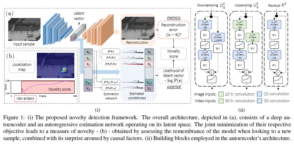
Our proposal contributes to the field by merging remembering and surprisal aspects into a unique framework: we design a generative unsupervised model (i.e., an autoencoder, represented in Fig. 1i) that exploits end-to-end training in order to maximize remembering effectiveness for normal samples whilst minimizing the surprisal of their latent representation.
This latter point is enabled by the maximization of the likelihood of latent representations through an autoregressive density estimator, which is performed in conjunction with the reconstruction error minimization.
We show that, by optimizing both terms jointly, the model implicitly seeks for minimum entropy representations maintaining its remembering/reconstructive power.
While entropy minimization approaches have been adopted in deep neural compression [3], to our knowledge this is the first proposal tailored for novelty detection.
In memory terms, our procedure resembles the concept of prototyping the normality using as few templates as possible.
Moreover, evaluating the output of the estimator enables the assessment of the surprisal aroused by a given sample.

우리의 제안은 remembering과 surprisal 측면을 unique framework로 병합함으로써 현장에 기여한다: 우리는 normal samples에 대한 기억 효과를 최대화하는 동시에 latent representation의 surprisal을 최소화하기 위해 end-to-end training을 활용하는 generative unsupervised model(즉, Fig. 1i에 표시된 autoencoder)을 설계한다.
이 후자 포인트는 reconstruction error 최소화와 함께 수행되는 autoregressive density estimator를 통해 latent representations의 likelihood를 최대화함으로써 활성화된다.
우리는 두 terms을 jointly 최적화함으로써, model이 암묵적으로 remembering/reconstructive 능력을 유지하는 minimum entropy representations을 추구한다는 것을 보여준다.
엔트로피 최소화 접근법이 deep neural compression [3]에서 채택되었지만, 우리가 아는 바로는 이것이 novelty detection에 첫 번째 맞춤 제안이다.
memory terms에, 우리의 procedure은 가능한 한 적은 템플릿을 사용하여 normality을 prototyping하는 개념과 유사하다.
또한 estimator의 output을 평가하면 주어진 sample에 의해 유발된 surprisal의 평가가 가능하다.

2. Related work

Reconstruction-based methods.
On the one hand, many works lean toward learning a parametric projection and reconstruction of normal data, assuming outliers will yield higher residuals.
Traditional sparse-coding algorithms [45, 9, 24] adhere to such framework, and represent normal patterns as a linear combination of a few basis components, under the hypotheses that novel examples would exhibit a non-sparse representation in the learned subspace.
In recent works, the projection step is typically drawn from deep autoencoders [11].
In [27] the authors recover sparse coding principles by imposing a sparsity regularization over the learned representations, while a recurrent neural network enforces their smoothness along the time dimension.
In [34], instead, the authors take advantage of an adversarial framework in which a discriminator network is employed as the actual novelty detector, spotting anomalies by performing a discrete in-distribution test.
Oppositely, future frame prediction [23] maximizes the expectation of the next frame exploiting its knowledge of the past ones; at test time, observed deviations against the predicted content advise for abnormality.
Differently from the above-mentioned works, our proposal relies on modeling the prior distribution of latent representations.
This choice is coherent with recent works from the density estimation community [38, 6].
However, to the best of our knowledge, our work is the first advocating for the importance of such a design choice for novelty detection.

Reconstruction-based methods. 한편, 많은 연구는 outliers가 더 높은 residuals를 산출한다고 가정하여 normal data의 parametric projection 및 reconstruction을 학습하는 데 기울고 있습니다.
Traditional sparse-coding algorithms [45, 9, 24]은 그러한 framework를 고수하며, novel examples가 학습된 subspace에서 non-sparse representation을 나타낸다는 hypotheses 아래 몇 가지 basis components의 linear combination으로 normal patterns을 나타낸다.
최근 연구에서 projection 단계는 일반적으로 deep autoencoders [11]에서 도출된다.
[27]에서 저자는 학습된 representations에 sparsity regularization을 부과하여 sparse coding principles을 recover하는 한편, recurrent neural network은 시간 차원을 따라 smoothness을 시행한다.
[34]에서 대신, 저자는 discriminator network가 실제 novelty detector로 사용되는 adversarial framework를 활용하여 discrete in-distribution test를 수행하여 anomalies를 포착한다.
반대로, future frame prediction[23]은 past frame에 대한 지식을 활용하는 next frame에 대한 expectation을 최대화한다; 테스트 시간에 predicted content에 대한 관측된 deviations는 abnormality에 advise한다.
위에서 언급한 연구와 달리, 우리의 제안은 latent representations의 prior distribution를 모델링하는 데 의존한다.
이러한 선택은 density estimation community [38, 6]의 최근 연구와 일관된다.
그러나 우리가 아는 한, 우리의 작업은 novelty detection을 위한 그러한 설계 선택의 중요성에 대한 첫번째 주장이다.

Probabilistic methods.
A complementary line of research investigates different strategies to approximate the density function of normal appearance and motion features.
The primary issue raising in this field concerns how to estimate such densities in a high-dimensional and complex feature space.
In this respect, prior works involve handcrafted features such as optical flow or trajectory analysis and, on top of that, employ both non-parametric [1] and parametric [5, 28, 22] estimators, as well as graphical modeling [16, 20].
Modern approaches rely on deep representations (e.g., captured by autoencoders), as in Gaussian classifiers [33] and Gaussian Mixtures [46].
In [13] the authors involve a Kernel Density Estimator (KDE) modeling activations from an auxiliary object detection network.
A recent research trend considers training Generative Adversarial Networks (GANs) on normal samples.
However, as such models approximate an implicit density function, they can be queried for new samples but not for likelihood values.
Therefore, GAN-based models employ different heuristics for the evaluation of novelty.
For instance, in [35] a guided latent space search is exploited to infer it, whereas [32] directly queries the discriminator for a normality score.

Probabilistic methods. 보완적인 연구 라인은 normal appearance와 motion features의 density function을 근사하기 위한 다양한 전략을 조사한다.
이 분야에서 제기되는 주요 문제는 고차원적이고 복잡한 feature space에서 그러한 밀도를 추정하는 방법에 관한 것이다.
이러한 측면에서 이전 연구는 optical flow 또는 궤적 분석과 같은 handcrafted features을 포함하며, 그 외에도 비모수 [1] 및 모수 [5, 28, 22] estimators와 graphical modeling [16, 20]을 모두 사용한다.
현대의 접근 방식은 Gaussian classifiers [33] 및 Gaussian Mixtures [46]에서와 같이 deep representations(예: autoencoders에 의한 캡처)에 의존한다.
[13]에서 저자는 auxiliary object detection network의 Kernel Density Estimator(KDE) modeling activations를 포함한다.
최근의 연구 경향은 normal samples에 대한 GAN(Generative Adversarial Network) 훈련을 고려한다.
그러나 이러한 모델은 implicit density function에 근사하므로 새로운 표본에 대해 쿼리할 수 있지만 likelihood values은 쿼리할 수 없다.
따라서 GAN-based models은 novelty 평가를 위해 서로 다른 heuristics을 사용한다.
예를 들어 [35]에서는 guided latent space search가 이를 추론하기 위해 이용되는 반면, [32]에서는 discriminator에 normality score를 직접 쿼리한다.

3. Proposed model

Maximizing the probability of latent representations is analogous to lowering the surprisal of the model for a normal configuration, defined as the negative log-density of a latent variable instance [39].
Conversely, remembering capabilities can be evaluated by the reconstruction accuracy of a given sample under its latent representation.

latent representations의 probability를 최대화하는 것은 latent variable instance [39]의 negative log-density로 정의되는 normal configuration에 대한 model의 surprisal을 낮추는 것과 유사하다.
반대로 기억 능력은 latent representation 하에서 given sample의 reconstruction accuracy로 평가할 수 있다.

We model the aforementioned aspects in a latent variable model setting, where the density function of training samples \(p(\mathbf{x})\) is modeled through an auxiliary random variable z, describing the set of causal factors underlying all observations.

우리는 앞에서 언급한 측면을 latent variable model setting에서 모델링하는데, 여기서 training samples \(p(\mathbf{x})\)의 밀도 함수는 auxiliary random variable z를 통해 모델링되며, 모든 관찰의 기반이 되는 일련의 인과적 요인을 설명한다.

By factorizing \[p(\mathbf{x}) = \int p(\mathbf{x}|\mathbf{z})p(\mathbf{z})d\mathbf{z} \qquad \qquad (1)\]

,where \(p(\mathbf{x}\vert \mathbf{z})\) is the conditional likelihood of the observation given a latent representation \(\mathbf{z}\) with prior distribution \(p(\mathbf{z})\), we can explicit both the memory and surprisal contribution to novelty.

\(\mathbf{z}\) : latent representation
\(p(\mathbf{z})\) : prior distribution of latent vector z
\(p(\mathbf{x}|\mathbf{z})\) : observation given z의 conditional likelihood
우리는 novelty에 memory contribution과 surprisal contribution 모두 명시한다.

We approximate the marginalization by means of an inference model responsible for the identification of latent space vector for which the contribution of \(p(\mathbf{x}\vert \mathbf{z})\) is maximal.

\(p(\mathbf{x}\vert \mathbf{z})\)의 contribution이 최대인 latent space vector의 identification을 담당하는 inference model을 사용하여 marginalization을 근사화한다.

Formally, we employ a deep autoencoder, in which the reconstruction error plays the role of the negative logarithm of \(p(\mathbf{x}\vert \mathbf{z})\), under the hypothesis that \(p(\mathbf{x}\vert \mathbf{z}) = \mathcal{N}(x\vert \tilde{x}, I)\) where \(\tilde{x}\) denotes the output reconstruction.

\(\tilde{x}\)이 output reconstruction인 hypothesis \(p(\mathbf{x}\vert \mathbf{z}) = \mathcal{N}(x\vert \tilde{x}, I)\)에서 reconstruction error가 \(p(\mathbf{x}\|\mathbf{z})\)의 negative logarithm 역할을 하는 deep autoencoder를 사용한다. \(\tilde{x}\) : output reconstruction

Additionally, surprisal is injected in the process by equipping the autoencoder with an auxiliary deep parametric estimator learning the prior distribution \(p(\mathbf{z})\) of latent vectors, and training it by means of Maximum Likelihood Estimation (MLE).

또한, autoencoder에 latent vectors의 prior distribution \(p(\mathbf{z})\)를 학습하는 auxiliary deep parametric estimator를 장착하고 Maximum Likelihood Estimation(MLE)을 통해 이를 훈련시킴으로써 이 과정에서 surprisal이 주입된다.

Our architecture is therefore composed of three building blocks (Fig. 1i): an encoder \(f(x; \theta_f )\), a decoder \(g(z; \theta_g)\) and a probabilistic model \(h(z; \theta_h)\): \[f(x; \theta_f) : \mathbb{R^m} → \mathbb{R^d}, g(z; \theta_{g}) : \mathbb{d} → \mathbb{m}, h(z; \theta_h): \mathbb{R^d} → [0,1].\]

우리의 architecture는 3개의 building blocks (Fig. 1i)를 구성한다 :
\(f(x; \theta_f )\) : encoder
\(g(z; \theta_g)\) : decoder
\(h(z; \theta_h)\) : probabilistic model

The encoder processes input \(x\) and maps it into a compressed representation \(z = f(x; \theta_{f} )\), whereas
the decoder provides a reconstructed version of the input \(\tilde{x} = g(z; \theta_{g})\).
The probabilistic model \(h(z; \theta_h)\) estimates the density in \(\mathbf{z}\) via an autoregressive process, allowing to avoid the adoption of a specific family of distributions (i.e., Gaussian), potentially unrewarding for the task at hand.
On this latter point, please refer to supplementary materials for comparison w.r.t. variational autoencoders [17].

encoder는 input \(x\)를 처리하고 이를 compressed representation \(z = f(x; \theta_{f} )\)로 매핑하는 반면,
decoder는 input \(\tilde{x} = g(z; \theta_{g})\)의 재구성 버전을 제공한다.
probabilistic model \(h(z; \theta_h)\)은 autoregressive process를 통해 \(\mathbf{z}\)의 density를 추정하여, 당면한 task에 대한 potentially unrewarding한 특정 분포 계열(즉, Gaussian)의 채택을 피할 수 있다.
이 latter point에 대해서는 variational autoencoders[17]에 대한 비교를 위한 보충 자료를 참조해 주십시오 [17].

With such modules, at test time, we can assess the two sources of novelty:
elements whose observation is poorly explained by the causal factors inducted by normal samples (i.e., high reconstruction error);
elements exhibiting good reconstructions whilst showing surprising underlying representations under the learned prior.

그러한 모듈을 사용하여, 테스트 시간에, 우리는 novelty의 두 가지 sources를 평가할 수 있다:
normal samples에 의해 유발된 인과 요소에 의해 관찰이 제대로 설명되지 않는 elements(즉, high reconstruction error);
좋은 reconstructions를 보여주는 elements이며 학습된 prior의 underlying representations을 보여준다.

Autoregressive density estimation.
Autoregressive models provide a general formulation for tasks involving sequential predictions, in which each output depends on previous observations [25, 29].
We adopt such a technique to factorize a joint distribution, thus avoiding to define its landscape a priori [21, 40].

Autoregressive models은 sequential predictions과 관련된 tasks에 대한 일반적인 공식을 제공하며, 각 출력은 이전 관찰에 따라 달라진다 [25, 29].
우리는 joint distribution를 factorize하기 위해 그러한 기술을 채택하여, 그 landscape를 priori(우선순위?)[21, 40]로 정의하는 것을 피한다.

Formally, \(p(\mathbf{z})\) is factorized as \[p(\mathbf{z}) = \prod_{i=1}^d p(z_i\vert\mathbf{z}_{<i}) \qquad \qquad (3)\]

so that estimating \(p(\mathbf{z})\) reduces to the estimation of each single Conditional Probability Density (CPD) expressed as \(p(z_i\vert \mathbf{z}_{<i})\), where the symbol \(<\) implies an order over random variables.

Some prior models obey handcrafted orderings [43, 42], whereas others rely on order agnostic training [41, 10].
Nevertheless, it is still not clear how to estimate the proper order for a given set of variables.
In our model, this issue is directly tackled by the optimization.
Indeed, since we perform auto-regression on learned latent representations, the MLE objective encourages the autoencoder to impose over them a pre-defined causal structure.
Empirical evidence of this phenomenon is given in the supplementary material.

From a technical perspective, the estimator \(h(z; theta_{h})\) outputs parameters for d distributions \(p(z_i\vert \mathbf{z}_{<i})\).
In our implementation, each CPD is modeled as a multinomial over B=100 quantization bins.
To ensure a conditional estimate of each underlying density, we design proper layers guaranteeing that the CPD of each symbol \(z_i\) is computed from inputs \(\{z_1, . . . , z_{i−1}\}\) only.

Objective and connection with differential entropy. The three components f, g and h are jointly trained to minimize \(\mathcal{L} ≡ \mathcal{L}(\theta_f , \theta_g, \theta_h)\) as follows:

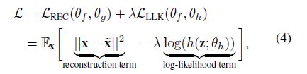,where \(\lambda\) is a hyper-parameter controlling the weight of the \(\mathcal{L}_{LLK}\) term. It is worth noting that it is possible to express the log-likelihood term as

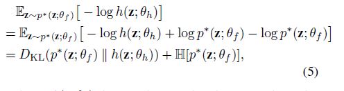
where \(p^*(\mathbf{z}; \theta_f )\) denotes the true distribution of the codes produced by the encoder, and is therefore parametrized by \(\theta_{f}\). This reformulation of the MLE objective yields meaningful insights about the entities involved in the optimization. On the one hand, the Kullback-Leibler divergence ensures that the information gap between our parametric model h and the true distribution \(p^*\) is small.
On the other hand, this framework leads to the minimization of the differential entropy of the distribution underlying the codes produced by the encoder \(f\).
Such constraint constitutes a crucial point when learning normality.
Intuitively, if we think about the encoder as a source emitting symbols (namely, the latent representations), its desired behavior, when modeling normal aspects in the data, should converge to a ‘boring’ process characterized by an intrinsic low entropy, since surprising and novel events are unlikely to arise during the training phase.
Accordingly, among all the possible settings of the hidden representations, the objective begs the encoder to exhibit a low differential entropy, leading to the extraction of features that are easily predictable, therefore common and recurrent within the training set.
This kind of features is indeed the most useful to distinguish novel samples from the normal ones, making our proposal a suitable regularizer in the anomaly detection setting.

We report empirical evidence of the decreasing differential entropy in Fig. 2, that compares the behavior of the same model under different regularization strategies.

3.1. Architectural Components

Autoencoder blocks.
Encoder and decoder are respectively composed by downsampling and upsampling residual blocks depicted in Fig. 1ii.
The encoder ends with fully connected (FC) layers.
When dealing with video inputs, we employ causal 3D convolutions [2] within the encoder (i.e., only accessing information from previous timesteps). Moreover, at the end of the encoder, we employ a temporally-shared full connection (TFC, namely a linear projection sharing parameters across the time axis on the input feature maps) resulting in a temporal series of feature vectors.
This way, the encoding procedure does not shuffle information across time-steps, ensuring temporal ordering.

Autoencoder blocks.
인코더와 디코더는 각각 그림 1ii에 설명된 다운샘플링 및 업샘플링 잔류 블록에 의해 구성된다.
인코더는 완전히 연결된(FC) 계층으로 끝납니다.
비디오 입력을 처리할 때, 우리는 인코더 내에서 인과적 3D 컨볼루션[2]을 사용한다(즉, 이전 시간 단계의 정보에만 액세스). 또한 인코더의 끝에는 임시 공유 전체 연결(TFC, 즉 입력 피처 맵의 시간 축에 걸친 선형 투영 공유 매개 변수)을 사용하여 시간적 일련의 피처 벡터를 생성한다.
이러한 방식으로 인코딩 절차는 시간 단계에 걸쳐 정보를 섞지 않으므로 시간적 순서가 보장된다.

Autoregressive layers.
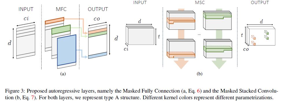
To guarantee the autoregressive nature of each output CPD, we need to ensure proper connectivity patterns in each layer of the estimator h. Moreover, since latent representations exhibit different shapes depending on the input nature (image or video), we propose two different solutions. When dealing with images, the encoder provides feature vectors with dimensionality \(d\).
The autoregressive estimator is composed by stacking multiple Masked Fully Connections (MFC, Fig. 3-(a)).
Formally, it computes output feature map \(\mathrm{o} \in \mathbb{R}^{d\times co}\) (where co is the number of output channels) given the input \(\mathrm{h} \in \mathbb{R}^{d\times ci}\) (assuming \(ci = 1\) at the input layer).
The connection between the input element \(h^k_i\) in position \(i\), channel \(k\) and the output element \(o^l_j\) is parametrized by

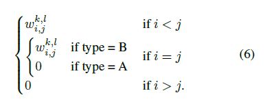
Type A forces a strict dependence on previous elements (and is employed only as the first estimator layer), whereas type B masks only succeeding elements.
Assuming each CPD modeled as a multinomial, the output of the last autoregressive layer (in \(\mathbb{R}^{d×B}\)) provides probability estimates for the B bins that compose the space quantization.

On the other hand, the compressed representation of video clips has dimensionality \(t \times d\), being t the number of temporal time-steps and d the length of the code.
Accordingly, the estimation network is designed to capture two-dimensional patterns within observed elements of the code.
However, naively plugging 2D convolutional layers would assume translation invariance on both axes of the input map, whereas, due to the way the compressed representation is built, this assumption is only correct along the temporal axis.
To cope with this, we apply d different convolutional kernels along the code axis, allowing the observation of the whole feature vector in the previous time-step as well as a portion of the current one.
Every convolution is free to stride along the time axis and captures temporal patterns.
In such operation, named Masked Stacked Convolution (MSC, Fig. 3-(b)), the \(i\)-th convolution is equipped with a kernel \(w^{(i)} \in \mathbb{R}^{3 \times d}\) kernel, that gets multiplied by the binary mask \(M^{(i)}\), defined as

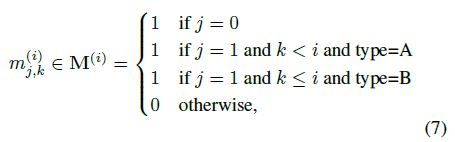
where j indexes the temporal axis and k the code axis.
Every single convolution yields a column vector, as a result of its stride along time.
The set of column vectors resulting from the application of the d convolutions to the input tensor \(h \in \mathbb{R}^{t \times d \times c_i}\) are horizontally stacked to build the output tensor \(\mathrm{o} ∈ \mathbb{R}^{t \times d \times co}\), as follows:

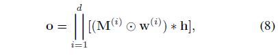
where \(\|\) represents the horizontal concatenation operation.

4. Experiments

We test our solution in three different settings: images, videos, and cognitive data.
In all experiments the novelty assessment on the \(i\)-th example is carried out by summing the reconstruction term (\(REC_i\)) and the log-likelihood term (\(LLK_i\)) in Eq. 4 in a single novelty score \(NS_i\):
\(NS_i=norm_S (REC_i) + norm_S (LLK_i.) \qquad \qquad (9)\)

Individual scores are normalized using a reference set of examples \(S\) (different for every experiment), \[norm_S(L_i) = \frac{L_i − max_{j \in S} L_j}{\max_{j \in S} L_j − \min{j \in S} L_j}. \; (10)\]

Further implementation details and architectural hyperparameters are in the supplementary material.

Code to reproduce results in this section is released at https://github.com/aimagelab/novelty-detection.

4.1. One-class novelty detection on images

To assess the model’s performances in one class settings, we train it on each class of either MNIST or CIFAR-10 separately.
In the test phase, we present the corresponding test set, which is composed of 10000 examples of all classes, and expect our model to assign a lower novelty score to images sharing the label with training samples.
We use standard train/test splits, and isolate 10% of training samples for validation purposes, and employ it as the normalization set (S in Eq. 9) for the computation of the novelty score.
As for the baselines, we consider the following:

한 클래스 설정에서 모델의 성능을 평가하기 위해 MNIST 또는 CIFAR-10의 각 클래스에서 별도로 학습한다.
테스트 단계에서, 우리는 모든 클래스의 10000개의 예제로 구성된 해당 테스트 세트를 제시하고, 우리의 모델이 훈련 샘플과 레이블을 공유하는 이미지에 더 낮은 새로움 점수를 할당할 것으로 기대한다.
우리는 표준 열차/테스트 분할을 사용하고, 검증 목적으로 훈련 샘플의 10%를 격리하고, 새로운 점수 계산을 위해 정규화 세트(S in Eq. 9)로 사용한다.
기준선의 경우 다음을 고려합니다.

• standard methods such as OC-SVM [36] and Kernel Density Estimator (KDE), employed out of features extracted by PCA-whitening;
• a denoising autoencoder (DAE) sharing the same architecture as our proposal, but defective of the density estimation module. The reconstruction error is employed as a measure of normality vs. novelty;
• a variational autoencoder (VAE) [17], also sharing the same architecture as our model, in which the Evidence Lower Bound (ELBO) is employed as the score;
• Pix-CNN [42], modeling the density by applying auto-regression directly in the image space;
• the GAN-based approach illustrated in [35].

We report the comparison in Tab. 1 in which performances are measured by the Area Under Receiver Operating Characteristic (AUROC), which is the standard metric for the task.
As the table shows, our proposal outperforms all baselines in both settings.

우리는 작업의 표준 메트릭인 AUROC(Area Under Receiver Operatic 특성)에 의해 성능이 측정되는 표 1에 비교를 보고한다.
표에서 알 수 있듯이, 우리의 제안은 두 가지 설정 모두에서 모든 기준을 능가한다.

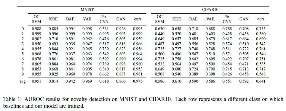
Considering MNIST, most methods perform favorably.
Notably, Pix-CNN fails in modeling distributions for all digits but one, possibly due to the complexity of modeling densities directly on pixel space and following a fixed autoregression order.
Such poor test performances are registered despite good quality samples that we observed during training: indeed, the weak correlation between sample quality and test log-likelihood of the model has been motivated in [37].
Surprisingly, OC-SVM outperforms most deep learning based models in this setting.

MNIST를 고려할 때 대부분의 방법은 양호한 성능을 보인다.
특히, Pix-CNN은 픽셀 공간에 직접 밀도를 모델링하고 고정 자기 회귀 순서를 따르는 복잡성으로 인해 한 자리만 제외하고 모든 자릿수에 대한 분포를 모델링하는 데 실패한다.
훈련 중에 관찰한 우수한 품질의 샘플에도 불구하고 이러한 테스트 성능이 등록된다. 실제로 모델의 샘플 품질과 테스트 로그 가능성 사이의 약한 상관관계가 [37]에서 동기 부여되었다.
놀랍게도, OC-SVM은 이 설정에서 대부분의 딥 러닝 기반 모델을 능가한다.

On the contrary, CIFAR10 represents a much more significant challenge, as testified by the low performances of most models, possibly due to the poor image resolution and visual clutter between classes.
Specifically, we observe that our proposal is the only model outperforming a simple KDE baseline; however, this finding should be put into perspective by considering the nature of non-parametric estimators.
Indeed, non-parametric models are allowed to access the whole training set for the evaluation of each sample.
Consequently, despite they benefit large sample sets in terms of density modeling, they lead into an unfeasible inference as the dataset grows in size.

반대로 CIFAR10은 대부분의 모델의 낮은 성능으로 증명된 바와 같이 훨씬 더 중요한 과제를 나타내는데, 이미지 해상도가 떨어지고 클래스 간의 시각적 혼란 때문일 수 있다.
구체적으로, 우리는 우리의 제안이 단순한 KDE 기준을 능가하는 유일한 모델이라는 것을 관찰한다. 그러나 이 발견은 비모수 추정기의 특성을 고려하여 관점에 두어야 한다.
실제로 비모수 모델은 각 샘플의 평가를 위해 전체 교육 세트에 액세스할 수 있다.
결과적으로, 밀도 모델링 측면에서 큰 샘플 세트에 이점이 있음에도 불구하고, 데이터 세트의 크기가 커짐에 따라 실현 불가능한 추론을 야기한다.

The possible reasons behind the difference in performance w.r.t. DAE are two-fold.
Firstly, DAE can recognize novel samples solely based on the reconstruction error, hence relying on its memorization capabilities, whereas our proposal also considers the likelihood of their representations under the learned prior, thus exploiting surprisal as well. Secondly, by minimizing the differential entropy of the latent distribution, our proposal increases the discriminative capability of the reconstruction.
Intuitively, this last statement can be motivated observing that novelty samples are forced to reside in a high probability region of the latent space, the latter bounded to solely capture unsurprising factors of variation arising from the training set.
On the other hand, the gap w.r.t. VAE suggests that, for the task at hand, a more flexible autoregressive prior should be preferred over the isotropic multivariate Gaussian.
On this last point, VAE seeks representations whose average surprisal converges to a fixed and expected value (i.e., the differential entropy of its prior), whereas our solution minimizes such quantity within its MLE objective.
This flexibility allows modulating the richness of the latent representation vs. the reconstructing capability of the model.
On the contrary, in VAEs, the fixed prior acts as a blind regularizer, potentially leading to over-smooth representations; this aspect is also appreciable when sampling from the model as shown in the supplementary material.

W.r.t.DAE의 성능 차이 이면에 있는 가능한 이유는 두 가지입니다.
첫째, DAE는 재구성 오류만을 기반으로 새로운 샘플을 인식할 수 있으므로 기억 능력에 의존할 수 있는 반면, 우리의 제안은 학습된 사전에서 이들의 표현 가능성을 고려하므로 놀라움도 활용한다. 둘째, 잠재 분포의 미분 엔트로피를 최소화함으로써 우리의 제안은 재구성의 차별적 능력을 증가시킨다.
직관적으로, 이 마지막 진술은 새로운 표본이 잠재 공간의 높은 확률 영역에 상주하도록 강요되고, 후자는 훈련 세트에서 발생하는 놀라운 변동 요인만 포착하도록 제한된다는 것을 관찰하는 동기가 될 수 있다.
반면, W.r.t. VAE는 당면한 작업의 경우 등방성 다변량 가우스보다 더 유연한 자기 회귀 사전이 선호되어야 한다고 제안한다.
이 마지막 점에서 VAE는 평균 놀라도가 고정 및 기대값(즉, 이전의 차등 엔트로피)으로 수렴되는 표현을 추구하는 반면, 우리의 솔루션은 MLE 목표 내에서 그러한 양을 최소화한다.
이러한 유연성은 잠재 표현의 풍부성 대 모델의 재구성 능력을 변조할 수 있다.
반대로 VAE에서는 고정식 사전이 블라인드 레귤레이터 역할을 하여 지나치게 매끄러운 표현을 할 수 있습니다. 이 측면은 보조 재료에 표시된 것처럼 모델로부터 표본을 추출할 때도 유용합니다.

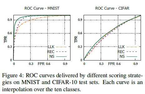
Fig. 4 reports an ablation study questioning the loss functions aggregation presented in Eq. 9. The figure illustrates ROC curves under three different novelty scores:
i) the log-likelihood term,
ii) the reconstruction term, and
iii) the proposed scheme that accounts for both.
As highlighted in the picture, accounting for both memorization and surprisal aspects is advantageous in each dataset.
Please refer to the supplementary material for additional evidence.

그림 4는 Eq. 9에 제시된 손실 함수 집계에 의문을 제기하는 절제 연구를 보고한다. 그림에는 세 가지 다른 신규성 점수의 ROC 곡선이 나와 있습니다.
i) 로그 우도 항,
ii) 재구성 용어 및
iii) 두 가지를 모두 설명하는 제안된 계획.
그림에서 강조했듯이, 암기와 놀라운 측면을 모두 설명하는 것은 각 데이터 세트에서 유리하다.
추가 증거는 보충 자료를 참고하세요.

4.2. Video anomaly detection

In video surveillance contexts, novelty is often considered in terms of abnormal human behavior.
Thus, we evaluate our proposal against state-of-the-art anomaly detection models.
For this purpose, we considered two standard benchmarks in literature, namely UCSD Ped2 [8] and ShanghaiTech [27].
Despite the differences in the number of videos and their resolution, they both contain anomalies that typically arise in surveillance scenarios (e.g., vehicles in pedestrian walkways, pick-pocketing, brawling).
For UCSD Ped, we preprocessed input clips of 16 frames to extract smaller patches (we refer to supplementary materials for details) and perturbed such inputs with random Gaussian noise with \(\sigma = 0.025\).
We compute the novelty score of each input clip as the mean novelty score among all patches.
Concerning ShanghaiTech, we removed the dependency on the scenario by estimating the foreground for each frame of a clip with a standard MOG-based approach and removing the background.
We fed the model with 16-frames clips, but ground-truth anomalies are labeled at frame level.

비디오 감시 컨텍스트에서, 새로움은 종종 비정상적인 인간 행동의 측면에서 고려된다.
따라서, 우리는 최신 이상 탐지 모델에 대해 우리의 제안을 평가한다.
이를 위해 문헌에서 UCSD Ped2[8]와 ShanghaiTech[27]의 두 가지 표준 벤치마크를 고려했습니다.
비디오 수와 해상도의 차이에도 불구하고, 둘 다 감시 시나리오에서 일반적으로 발생하는 이상 징후를 포함하고 있다(예: 보행자 통로의 차량, 소매치기, 싸움).
UCSD Ped의 경우, 우리는 더 작은 패치를 추출하기 위해 16프레임의 입력 클립을 사전 처리했으며(자세한 내용은 보조 자료를 참조), \(\sigma = 0.025\)의 무작위 가우스 노이즈로 그러한 입력을 교란시켰다.
우리는 모든 패치 중 평균 새로움 점수로 각 입력 클립의 새로움 점수를 계산한다.
상하이테크와 관련하여, 우리는 표준 MG 기반 접근법으로 클립의 각 프레임에 대한 전경을 추정하고 배경을 제거함으로써 시나리오에 대한 의존성을 제거했다.
모델에 16프레임 클립을 공급했지만, 지상 실측 이상 징후는 프레임 레벨에서 라벨링된다.

In order to recover the novelty score of each frame, we compute the mean score of all clips in which it appears.
We then merge the two terms of the loss function following the same strategy illustrated in Eq. 9, computing however normalization coefficients in a per-sequence basis, following the standard approach in the anomaly detection literature.
The scores for each sequence are then concatenated to compute the overall AUROC of the model.
Additionally, we envision localization strategies for both datasets.
To this aim, for UCSD, we denote a patch exhibiting the highest novelty score in a frame as anomalous.
Differently, in ShanghaiTech, we adopt a sliding-window approach [44]: as expected, when occluding the source of the anomaly with a rectangular patch, the novelty score drops significantly.
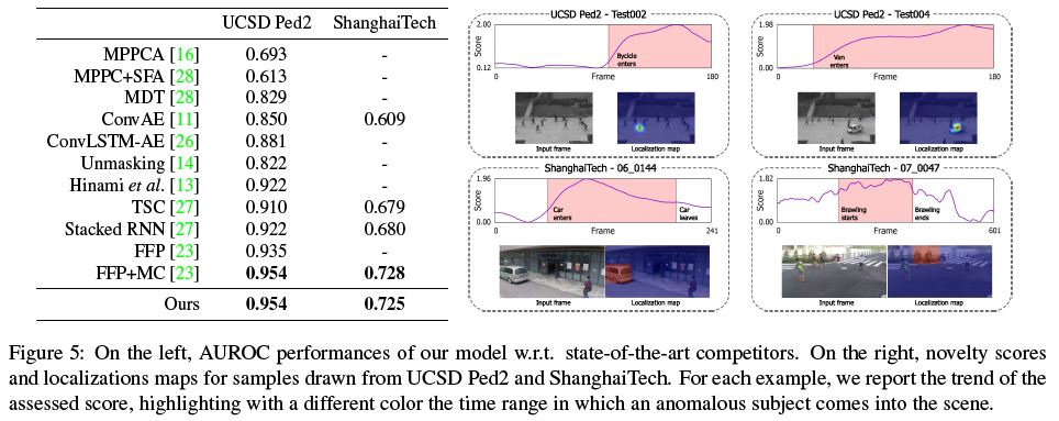
Fig. 5 reports results in comparison with prior works, along with qualitative assessments regarding the novelty score and localization capabilities.
Despite a more general formulation, our proposal scores on-par with the current state-of-the-art solutions specifically designed for video applications and taking advantage of optical flow estimation and motion constraints.
Indeed, in the absence of such hypotheses (FFP entry in Fig. 5), our method outperforms future frame prediction on UCSD Ped2.

각 프레임의 새로움 점수를 복구하기 위해 표시되는 모든 클립의 평균 점수를 계산합니다.
그런 다음 Eq. 9에 설명된 동일한 전략에 따라 손실 함수의 두 항을 병합하고, 이상 탐지 문헌의 표준 접근 방식을 따라 시퀀스별로 정규화 계수를 계산한다.
그런 다음 각 시퀀스에 대한 점수를 연결하여 모델의 전체 AUROC를 계산한다.
또한, 우리는 두 데이터 세트에 대한 지역화 전략을 구상한다.
이를 위해 UCSD의 경우 프레임에서 가장 높은 새로움 점수를 나타내는 패치를 이례적으로 나타낸다.
이와는 달리, 상하이 기술에서는 슬라이딩 윈도우 접근 방식을 채택한다[44]. 예상대로, 직사각형 패치로 이상 징후 근원을 차단하면 새로움 점수가 크게 떨어진다.
그림 5는 새로운 점수와 지역화 능력에 대한 정성적 평가와 함께 이전 연구와 비교한 결과를 보여준다.
보다 일반적인 공식에도 불구하고, 우리의 제안은 비디오 애플리케이션을 위해 특별히 설계된 최신 솔루션과 동등하게 평가되며 광학 흐름 추정 및 모션 제약 조건을 이용한다.
실제로, 그러한 가설(그림 5의 FFP 입력)이 없는 경우, 우리의 방법은 UCSD Ped2에서 미래 프레임 예측을 능가한다.

4.3. Model Analysis

CIFAR-10 with semantic features.
We investigate the behavior of our model in the presence of different assumptions regarding the expected nature of novel samples.
We expect that, as the correctness of such assumptions increases, novelty detection performances will scale accordingly.
Such a trait is particularly desirable for applications in which prior beliefs about novel examples can be envisioned.
To this end, we leverage the CIFAR-10 benchmark described in Sec. 4.1 and change the type of information provided as input.
Specifically, instead of raw images, we feed our model with semantic representations extracted by ResNet-50 [12], either pre-trained on Imagenet (i.e., assume semantic novelty) or CIFAR-10 itself (i.e., assume data-specific novelty).
The two models achieved respectively 79.26 and 95.4 top-1 classification accuracies on the respective test sets.
Even though this procedure is to be considered unfair in novelty detection, it serves as a sanity check delivering the upper-bound performances our model can achieve when applied to even better features.
To deal with dense inputs, we employ a fully connected autoencoder and MFC layers within the estimation network.

CIFAR-10 with semantic features.
우리는 새로운 샘플의 예상 특성에 관한 서로 다른 가정이 존재하는 상태에서 모델의 동작을 조사한다.
우리는 그러한 가정의 정확성이 증가함에 따라 새로운 감지 성능이 그에 따라 확장될 것으로 기대한다.
이러한 특성은 새로운 사례에 대한 사전 믿음이 구상될 수 있는 응용 분야에 특히 바람직하다.
이를 위해, 우리는 4.1절에서 설명한 CIFAR-10 벤치마크를 활용하고 입력으로 제공되는 정보의 유형을 변경한다.
구체적으로, 원시 이미지 대신, 우리는 ResNet-50[12]에 의해 추출된 의미 표현을 모델에 공급한다. 이미지넷에서 사전 훈련된 (즉, 의미적 새로움을 가정한다) 또는 CIFAR-10 자체(즉, 데이터별 새로움을 가정한다).
두 모델은 각 테스트 세트에서 각각 79.26과 95.4 상위 1등급 분류 정확도를 달성했다.
이 절차는 새로움 감지에서 불공정하다고 간주되지만, 훨씬 더 나은 기능에 적용될 때 우리 모델이 달성할 수 있는 상한 성능을 제공하는 온전성 검사 역할을 한다.
조밀한 입력을 처리하기 위해 추정 네트워크 내에서 완전히 연결된 자동 인코더와 MFC 계층을 사용한다.

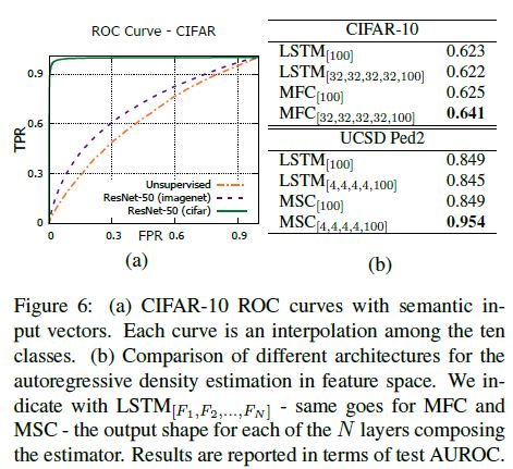
Fig. 6-(a) illustrates the resulting ROC curves, where semantic descriptors improve AUROC w.r.t. raw image inputs (entry “Unsupervised”).
Such results suggest that our model profitably takes advantage of the separation between normal and abnormal input representations and scales accordingly, even up to optimal performances for the task under consideration.
Nevertheless, it is interesting to note how different degrees of supervision deliver significantly different performances.
As expected, dataset-specific supervision increases the AUROC from 0.64 up to 0.99 (a perfect score).
Surprisingly, semantic feature vectors trained on Imagenet (which contains all CIFAR classes) provide a much lower boost, yielding an AUROC of 0.72.
Such result suggests that, even in the rare cases where the semantic of novelty can be known in advance, its contribution has a limited impact in modeling the normality, mostly because novelty can depend on other cues (e.g., low-level statistics).

그림 6-(a)는 의미론적 설명자가 AUROC w.r.t. 원시 이미지 입력을 개선하는 결과 ROC 곡선을 보여준다(항목 “비지도”).
그러한 결과는 우리의 모델이 정상적인 입력 표현과 비정상적인 입력 표현 사이의 분리를 수익적으로 활용하고 고려 중인 작업에 대한 최적의 성능까지 그에 따라 확장한다는 것을 시사한다.
그럼에도 불구하고, 서로 다른 수준의 감독이 유의하게 다른 성능을 제공하는 방법에 주목하는 것은 흥미롭다.
예상대로 데이터 세트별 감독은 AUROC를 0.64에서 0.99(만점)로 증가시킨다.
놀랍게도, Imagnet(모든 CIFAR 클래스를 포함)에서 훈련된 의미론적 특징 벡터는 훨씬 낮은 부스트를 제공하여 0.72의 AUROC를 산출한다.
그러한 결과는 새로움의 의미를 미리 알 수 있는 드문 경우에도, 새로움이 주로 다른 단서(예: 낮은 수준의 통계)에 의존할 수 있기 때문에 정규성을 모델링하는 데 그 기여도가 제한적이라는 것을 시사한다.

Autoregression via recurrent layers.
To measure the contribution of the proposed MFC and MSC layers described in Sec. 3, we test on CIFAR-10 and UCSD Ped2, alternative solutions for the autoregressive density estimator.
Specifically, we investigate recurrent networks, as they represent the most natural alternative featuring autoregressive properties.
We benchmark the proposed building blocks against an estimator composed of LSTM layers, which is designed to sequentially observe latent symbols \(z<i\) and output the CPD of \(z_i\) as the hidden state of the last layer.
We test MFC, MSC and LSTM in single-layer and multi-layer settings, and report all outcomes in Fig. 6-(b).

Autoregression via recurrent layers.
3항에서 설명하는 제안된 MFC 및 MSC 계층의 기여도를 측정하기 위해, 우리는 자기 회귀 밀도 추정기의 대안 솔루션인 CIFAR-10 및 UCSD Ped2에서 테스트한다.
구체적으로, 우리는 반복 네트워크가 자기 회귀 속성을 특징으로 하는 가장 자연스러운 대안을 나타내기 때문에 반복 네트워크를 조사한다.
우리는 LSTM 계층으로 구성된 추정기에 대해 제안된 빌딩 블록을 벤치마킹하는데, LSTM 계층은 잠재 기호 \(z<i\)를 순차적으로 관찰하고 마지막 계층의 숨겨진 상태로 CPD \(z_i\)를 출력하도록 설계되었다.
우리는 단일 계층 및 다중 계층 설정에서 MFC, MSC 및 LSTM을 테스트하고 모든 결과를 그림 6-(b)에 보고한다.

It emerges that, even though our solutions perform similarly to the recurrent baseline when employed in a shallow setting, they significantly take advantage of their depth when stacked in consecutive layers.
MFC and MSC, indeed, employ disentangled parametrizations for each output CPD.
This property is equivalent to the adoption of a specialized estimator network for each zi, thus increasing the proficiency in modeling the density of its designated CPD.
On the contrary, LSTM networks embed all the history (i.e., the observed symbols) in their memory cells, but manipulate each input of the sequence through the same weight matrices.
In such a regime, the recurrent module needs to learn parameters shared among symbols, losing specialization and eroding its modeling capabilities.

우리의 솔루션이 얕은 환경에서 사용될 때 반복 기준선과 유사하게 수행되지만 연속 레이어에 쌓일 때 깊이를 크게 활용한다는 사실이 밝혀졌다.
실제로 MFC와 MSC는 각 출력 CPD에 대해 분리된 매개 변수를 사용한다.
이 속성은 각 zi에 대해 전문화된 추정기 네트워크를 채택하는 것과 동일하므로, 지정된 CPD의 밀도를 모델링하는 숙련도가 증가한다.
반대로 LSTM 네트워크는 모든 기록(즉, 관찰된 기호)을 메모리 셀에 포함시키지만 동일한 가중치 행렬을 통해 시퀀스의 각 입력을 조작한다.
이러한 체제에서 반복 모듈은 기호 간에 공유되는 매개 변수를 학습하여 전문화를 상실하고 모델링 기능을 잠식할 필요가 있다.

4.4. Novelty in cognitive temporal processes

As a potential application of our proposal, we investigate its capability in modeling human attentional behavior.
To this end, we employ the DR(eye)VE dataset [30], introduced for the prediction of focus of attention in driving contexts.
It features 74 driving videos where frame-wise fixation maps are provided, highlighting the region of the scene attended by the driver.
In order to capture the dynamics of attentional patterns, we purposely discard the visual content of the scene and optimize our model on clips of fixation maps, randomly extracted from the training set.
After training, we rely on the novelty score of each clip as a proxy for the uncommonness of an attentional pattern.
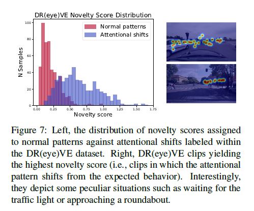
Moreover, since the dataset features annotations of peculiar and unfrequent patterns (such as distractions, recording errors), we can measure the correlation of the captured novelty w.r.t. those.
In terms of AUROC, our model scores 0.926, highlighting that novelty can arise from unexpected behaviors of the driver, such as distractions or other shifts in attention.
Fig. 7 reports the different distribution of novelty scores for ordinary and peculiar events.

우리의 제안의 잠재적인 적용으로, 우리는 인간의 주의 행동을 모델링하는 그것의 능력을 조사한다.
이를 위해 DR(눈)을 사용합니다.VE 데이터 세트[30]는 운전 컨텍스트에서 주의 집중을 예측하기 위해 도입되었다.
프레임별 고정 맵이 제공되는 74개의 주행 비디오가 담겨 있어 운전자가 참석하는 장면의 영역을 조명한다.
주의 패턴의 역학을 포착하기 위해, 우리는 훈련 세트에서 무작위로 추출한 고정 맵 클립에서 장면의 시각적 내용을 의도적으로 버리고 모델을 최적화한다.
훈련 후, 우리는 주의 패턴의 흔하지 않은 것에 대한 대리로서 각 클립의 신기한 점수에 의존한다.
또한 데이터 세트는 특이하고 빈번하지 않은 패턴의 주석(예: 산만, 기록 오류)을 특징으로 하므로 캡처된 새로움 w.r.t의 상관 관계를 측정할 수 있다.
AUROC의 관점에서, 우리의 모델은 0.926점을 기록하여, 새로움이 주의 집중력의 다른 이동과 같은 운전자의 예상치 못한 행동에서 발생할 수 있음을 강조한다.
그림 7은 일반 이벤트와 특이한 이벤트에 대한 새로운 점수의 다른 분포를 보고한다.

5. Conclusions

We propose a comprehensive framework for novelty detection.
We formalize our model to capture the twofold nature of novelties, which concerns the incapability to remember unseen data and the surprisal aroused by the observation of their latent representations.
From a technical perspective, both terms are modeled by a deep generative autoencoder, paired with an additional autoregressive density estimator learning the distribution of latent vectors by maximum likelihood principles.
To this aim, we introduce two different masked layers suitable for image and video data.
We show that the introduction of such an auxiliary module, operating in latent space, leads to the minimization of the encoder’s differential entropy, which proves to be a suitable regularizer for the task at hand.
Experimental results show state-of-the-art performances in one-class and anomaly detection settings, fostering the flexibility of our framework for different tasks without making any data-related assumption.

우리는 novelty detection를 위한 포괄적인 프레임워크를 제안한다.
우리는 보이지 않는 데이터를 기억하는 능력과 잠재 표현의 관찰에 의해 유발되는 놀라움과 관련된 새로운 것의 두 가지 특성을 포착하기 위해 우리의 모델을 공식화한다.
기술적 관점에서 두 용어는 최대우도 원리에 의한 잠재 벡터의 분포를 학습하는 추가 자기 회귀 밀도 추정기와 쌍으로 구성된 심층 생성 자동 인코더에 의해 모델링된다.
이를 위해 이미지 및 비디오 데이터에 적합한 두 가지 마스킹된 레이어를 소개한다.
우리는 잠재 공간에서 작동하는 그러한 보조 모듈의 도입이 인코더의 미분 엔트로피를 최소화하도록 이끌며, 이는 당면한 작업에 적합한 정규화라는 것을 보여준다.
실험 결과는 1등급 및 이상 탐지 설정에서 최첨단 성능을 보여 데이터 관련 가정을 하지 않고 다양한 작업에 대한 프레임워크의 유연성을 강화한다.

Acknowledgements.

We gratefully acknowledge Facebook Artificial Intelligence Research and Panasonic Silicon Valley Lab for the donation of GPUs used for this research.