2018 paper

Stanislav Pidhorskyi Ranya Almohsen
Donald A. Adjeroh
Gianfranco Doretto

Lane Department of Computer Science and Electrical Engineering West Virginia University,Morgantown,WV 26506

---

참고할만한 블로그1
참고할만한 블로그2
매니폴드
VAE AAE AutoEncoder의 모든것

---

• ABSTRACT
• 1 Introduction
• 2 Related Work
  • 3 Generative Probabilistic Novelty Detection
  • 3.1 Computing the distribution of data samples
• 4 Manifold learning with adversarial autoencoders
  • 4.1 Adversarial losses
  • 4.2 Autoencoder loss
  • 4.3 Full objective
• 5 Implementation Details and Complexity
• 6 Experiments
  • 6.1 Datasets
  • 6.2 Results
  • 6.3 Ablation
• 7 Conclusion
  • Acknowledgments

ABSTRACT

Novelty detection is the problem of identifying whether a new data point is considered to be an inlier or an outlier.
We assume that training data is available to describe only the inlier distribution.
Recent approaches primarily leverage deep encoder-decoder network architectures to compute a reconstruction error that is used to either compute a novelty score or to train a one-class classifier.
While we too leverage a novel network of that kind, we take a probabilistic approach and effectively compute how likely it is that a sample was generated by the inlier distribution.
We achieve this with two main contributions.

First, we make the computation of the novelty probability feasible because we linearize the parameterized manifold capturing the underlying structure of the inlier distribution, and show how the probability factorizes and can be computed with respect to local coordinates of the manifold tangent space.

Second, we improve the training of the autoencoder network.
An extensive set of results show that the approach achieves state-of-the-art performance on several benchmark datasets.

Novelty detection은 new data point이 inlier인지 outlier인지로 간주되는지 여부를 식별하는 문제이다.
우리는 training data가 inlier distribution만 설명할 수 있다고 가정한다.
최근의 접근 방식은 주로 deep encoder-decoder network 아키텍처를 활용하여 novelty score를 계산하거나 one-class classifier를 train시키는 데 사용되는 reconstruction error를 계산한다.
우리도 그러한 종류의 novel network를 활용하지만 probabilistic 접근법을 취하여 inlier distribution에 의해 sample이 generate되었을 가능성을 효과적으로 계산한다.
우리는 두 가지 main contributions로 이것을 달성한다.

첫째, inlier distribution의 기본 구조를 캡처하는 매개 변수화된 manifold를 linearize하고, manifold tangent space의 local coordinates에 대해 probability을 어떻게 factorizes(분해)하고 계산할 수 있는지 보여주기 때문에 novelty probability 계산을 가능(feasible)하게 한다.

둘째, autoencoder network의 training을 개선한다.
광범위한 결과 집합은 이 접근 방식이 여러 benchmark datasets에서 state-of-the-art 성능을 달성한다는 것을 보여준다.

1 Introduction

Novelty detection is the problem of identifying whether a new data point is considered to be an inlier or an outlier.
From a statistical point of view this process usually occurs while prior knowledge of the distribution of inliers is the only information available.
This is also the most difficult and relevant scenario because outliers are often very rare, or even dangerous to experience (e.g., in industry process fault detection [1]), and there is a need to rely only on inlier training data.
Novelty detection has received significant attention in application areas such as medical diagnoses [2], drug discovery [3], and among others, several computer vision applications, such as anomaly detection in images [4, 5], videos [6], and outlier detection [7, 8].
We refer to [9] for a general review on novelty detection.
The most recent approaches are based on learning deep network architectures [10, 11], and they tend to either learn a one-class classifier [12, 11], or to somehow leverage as novelty score, the reconstruction error of the encoder-decoder architecture they are based on [13, 7].

Novelty detection은 new data point가 inlier인지 outlier인지로 간주되는지 여부를 식별하는 문제이다.
통계적인 관점에서 이 프로세스는 distribution of inliers에 대한 사전 지식이 이용 가능한 information이면 발생한다.
outliers는 종종 매우 희귀하거나 심지어 경험하기 위험하기 때문에(예: 산업 프로세스 결함 감지 [1]) 가장 어렵고 관련성이 높은 시나리오이기도 하다, 그래서 inlier training data에 의존할 필요가 있다.
Novelty detection는 의학 진단[2], 약물 발견[3]과 같은 응용 분야에서 상당한 관심을 받았고, 그 중에서도 이미지[4, 5], 비디오[6], anomaly detection[7, 8]와 같은 여러 컴퓨터 비전 응용 분야에서 주목을 받았다.
우리는 novelty detection에 대한 general review를 위해 [9]를 참조한다.
가장 최근의 접근 방식은 deep network 아키텍처 학습[10, 11]을 기반으로 하며, one-class classifier [12, 11]를 학습하거나, [13, 7]에 기반한 encoder-decoder아키텍처의 reconstruction error, novelty score로 활용하는 경향이 있다.

In this work, we introduce a new encoder-decoder architecture as well, which is based on adversarial autoencoders [14].
However, we do not train a one-class classifier, instead, we learn the probability distribution of the inliers.
Therefore, the novelty test simply becomes the evaluation of the probability of a test sample, and rare samples (outliers) fall below a given threshold.
We show that this approach allows us to effectively use the decoder network to learn the parameterized manifold shaping the inlier distribution, in conjunction with the probability distribution of the (parameterizing) latent space.
The approach is made computationally feasible because for a given test sample we linearize the manifold, and show that with respect to the local manifold coordinates the data model distribution factorizes into a component dependent on the manifold (decoder network plus latent distribution), and another one dependent on the noise, which can also be learned offline.

본 연구에서는 adversarial autoencoders[14]를 기반으로 하는 새로운 encoder-decoder 아키텍처도 소개한다.
그러나 우리는 one-class classifier를 훈련시키지 않고 대신, inliers의 probability distribution를 학습한다.
따라서 novelty test는 단순히 test sample의 probability에 대한 evaluation이 되며, rare samples(outliers)는 지정된 threshold 아래로 떨어진다.
우리는 이 접근법이 decoder network를 효과적으로 사용하여 (parameterizing)latent space의 probability distribution와 함께 inlier distribution를 형성하는 매개 변수화된 manifold를 학습할 수 있음을 보여준다.
이 접근 방식은 주어진 test sample에 대해 manifold를 linearize하고, local manifold coordinates에 대하여 data model distribution가 manifold에 종속된 component(decoder network plus latent distribution)로 factorize되고, offline 학습될 수 있는 noise에 종속된다는 것을 보여주기 때문에 계산적으로 가능하다.

32nd Conference on Neural Information Processing Systems (NIPS 2018), Montréal, Canada.
We named the approach generative probabilistic novelty detection (GPND) because we compute the probability distribution of the full model, which includes the signal plus noise portion, and because it relies on being able to also generate data samples.
We are mostly concerned with novelty detection using images, and with controlling the distribution of the latent space to ensure good generative reproduction of the inlier distribution.
This is essential not so much to ensure good image generation, but for the correct computation of the novelty score.
This aspect has been overlooked by the deep learning literature so far, since the focus has been only on leveraging the reconstruction error.
We do leverage that as well, but we show in our framework that the reconstruction error affects only the noise portion of the model.
In order to control the latent distribution and image generation we learn an adversarial autoencoder network with two discriminators that address these two issues.

제32차 Conference on Neural Information Processing Systems (NIPS 2018), Montréal, Canada.
signal plus noise 부분을 포함하는 전체 모델의 probability distribution를 계산하고 data samples도 generate할 수 있는 것에 의존하기 때문에, approach를 generative probabilistic novelty detection (GPND)라고 이름 지었다.
우리는 대부분 이미지를 사용한 novelty detection과 inlier distribution의 좋은 generative reproduction을 보장하기 위해 latent space의 distribution를 제어하는 것에 관심이 있다.
이것은 좋은 이미지 generation을 보장하기 위해서만이 아니라 novelty score의 정확한 계산을 위해서도 필수적이다.
reconstruction error를 활용하는 데만 초점이 맞춰져 있었기 때문에, 이러한 측면은 지금까지 deep learning literature에서 간과되어 왔다.
우리도 이 점을 활용하지만, reconstruction error가 model의 noise 부분에만 영향을 미친다는 것을 framework에서 보여준다.
latent distribution와 image generation을 제어하기 위해 우리는 이 두 문제를 해결하는 두 개의 discriminators가 있는 adversarial autoencoder network를 학습한다.

Section 2 reviews the related work.
Section 3 introduces the GPND framework, and
Section 4 describes the training and architecture of the adversarial autoencoder network.
Section 6 shows a rich set of experiments showing that GPND is very effective and produces state-of-the-art results on several benchmarks.

Section 2는 related work를 검토한다.
Section 3은 GPND framework를 소개하고,
Section 4는 adversarial autoencoder network의 training과 아키텍처를 설명한다.
Section 6은 GPND가 매우 효과적이며 여러 benchmarks에서 tate-of-the-art 결과를 산출한다는 것을 보여주는 풍부한 실험 세트를 보여준다.

2 Related Work

Novelty detection is the task of recognizing abnormality in data.
The literature in this area is sizable.
Novelty detection methods can be statistical and probabilistic based [15, 16], distance based [17], and also based on self-representation [8].
Recently, deep learning approaches [7, 11] have also been used, greatly improving the performance of novelty detection.

Novelty detection은 data의 abnormality를 인식하는 작업이다.
이 지역의 literature은 상당한 규모이다.
Novelty detection은 statistical 및 probabilistic based[15, 16], distance based [17], self-representation에 기반할 수 있다[8].
최근에는 deep learning approaches[7, 11]도 사용되어 novelty detection을 크게 향상시켰다.

Statistical methods [18, 19, 15, 16] usually focus on modeling the distribution of inliers by learning the parameters defining the probability, and outliers are identified as those having low probability under the learned model.
Distance based outlier detection methods [20, 17, 21] identify outliers by their distance to neighboring examples.
They assume that inliers are close to each other while the abnormal samples are far from their nearest neighbors.
A known work in this category is LOF [22], which is based on k-nearest neighbors and density based estimation.
More recently, [23] introduced the Kernel Null Foley-Sammon Transform (KNFST) for multi-class novelty detection, where training samples of each known category are projected onto a single point in the null space and then distances between the projection of a test sample and the class representatives are used to obtain a novelty measure.
[24] improves on previous approaches by proposing an incremental procedure called Incremental Kernel Null Space Based Discriminant Analysis (IKNDA).

통계적 방법[18, 19, 15, 16]은 일반적으로 확률을 정의하는 매개 변수를 학습하여 inliers의 distribution를 modeling하는 데 초점을 맞추고 있으며, outliers는 학습된 model에서 낮은 probability를 가진 것으로 식별된다.
Distance 기반 outlier detection 방법[20, 17, 21]은 outliers를 neighboring examples까지의 distance로 식별한다. inliers는 서로 가깝지만 abnormal samples는 nearest neighbors과 멀리 떨어져 있다고 가정한다.
이 category의 known work는 k-nearest neighbors과 density based estimation을 기반으로 하는 LOF [22]이다.
보다 최근에 [23]은 multi-class novelty detection를 위한 Kernel Null Foley-Sammon Transform (KNFST)을 도입했는데, 여기서 알려진 각 category의 training samples이 null space의 single point에 projected된 다음 test sample projection과 class representatives 사이의 distances가 novelty measure을 얻기 위해 사용된다.
[24]는 Incremental Kernel Null Space Based Discriminant Analysis (IKNDA)로 불리는 incremental procedure를 제안하여 이전 approaches을 개선한다.

Since outliers do not have sparse representations, self-representation approaches have been proposed for outlier detection in a union of subspaces [4, 25].
Similarly, deep learning based approaches have used neural networks and leveraged the reconstruction error of encoder-decoder architectures.
[26, 27] used deep learning based autoencoders to learn the model of normal behaviors and employed a reconstruction loss to detect outliers.
[28] used a GAN [29] based method by generating new samples similar to the training data, and demonstrated its ability to describe the training data.
Then it transformed the implicit data description of normal data to a novelty score.
[10] trained GANs using optical flow images to learn a representation of scenes in videos.
[7] minimized the reconstruction error of an autoencoder to remove outliers from noisy data, and by utilizing the gradient magnitude of the auto-encoder they make the reconstruction error more discriminative for positive samples.
In [11] they proposed a framework for one-class classification and novelty detection.
It consists of two main modules learned in an adversarial fashion.
The first is a decoder-encoder convolutional neural network trained to reconstruct inliers accurately, while the second is a one-class classifier made with another network that produces the novelty score.

outliers는 sparse representations을 가지고 있지 않기 때문에, union of subspaces에서 outlier detection에 대해 self-representation approaches가 제안되었다.[4, 25]
마찬가지로 deep learning 기반 approaches는 neural networks를 사용하고 encoder-decoder 아키텍처의 reconstruction error를 활용했다.
[26, 27]은 deep learning 기반 autoencoders를 사용하여 normal behaviors의 model를 학습하고 reconstruction loss를 사용하여 outliers를 탐지했다.
[28]은 training data와 유사한 새로운 samples를 generate하는 GAN [29] 기반 method를 사용했으며, training data를 설명하는 능력을 입증했다.
그런 다음 normal data에 대한 암묵적 data 설명을 novelty score로 변환했다.
[10]은 optical flow images를 사용하여 비디오 장면의 representation을 학습하는 GAN을 훈련시켰다.
[7]은 autoencoder의 reconstruction error를 최소화하여 noisy data에서 outliers를 제거했으며, auto-encoder의 기울기 크기(gradient magnitude)를 활용하여 positive samples에 대한 reconstruction error를 보다 차별화(discriminative)할 수 있다.
[11]에서 그들은 one-class classification과 novelty detection을 위한 framework를 제안했다.
이것은 adversarial 방식으로 학습된 두 가지 주요 모듈로 구성된다.
첫 번째는 inliers를 정확하게 reconstruct하도록 훈련된 decoder-encoder convolutional neural network이고,
두 번째는 novelty score를 생성하는 또 다른 network로 만들어진 one-class classifier이다.

The proposed approach relates to the statistical methods because it aims at computing the probability distribution of test samples as novelty score, but it does so by learning the manifold structure of the distribution with an encoder-decoder network.
Moreover, the method is different from those that learn a one-class classifier, or rely on the reconstruction error to compute the novelty score, because in our framework we represent only one component of the score computation, allowing to achieve an improved performance.

제안된 approach는 test samples의 probability distribution을 novelty score로 계산하는 것을 목표로 하기 때문에 statistical methods와 관련이 있지만, encoder-decoder network를 통해 distribution의 manifold structure을 학습함으로써 관련된다.
또한, 이 method는 one-class classifier를 학습하거나 reconstruction error에 의존하여 novelty score를 계산하는 방법과 다르다, 왜냐하면 우리의 framework에서 우리는 score 계산의 한 component만 나타내므로 향상된 성능을 달성할 수 있기 때문이다.

State-of-the art works on density estimation for image compression include Pixel Recurrent Neural Networks [30] and derivatives [31, 32].
These pixel-based methods allow to sequentially predict pixels in an image along the two spatial dimensions.
Because they model the joint distribution of the raw pixels along with their sequential correlation, it is possible to use them for image compression.
Although they could also model the probability distribution of known samples, they work at a local scale in a patch-based fashion, which makes non-local pixels loosely correlated.
Our approach instead, does not allow modeling the probability density of individual pixels but works with the whole image.
It is not suitable for image compression, and while its generative nature allows in principle to produce novel images, in this work we focus only on novelty detection by evaluating the inlier probability distribution on test samples.

이미지 압축을 위한 density estimation에 대한 State-of-the art 작업에는 Pixel Recurrent Neural Networks [30]과 파생 모델[31,32]이 포함된다.
이러한 pixel-based methods을 사용하면 두 spatial dimensions을 따라 이미지의 픽셀을 순차적으로 예측할 수 있다.
raw pixels의 joint distribution를 순차적 상관 관계(sequential correlation)와 함께 모델링하기 때문에, image 압축에 사용할 수 있다.
known samples의 probability distribution를 모델링할 수도 있지만, patch-based 방식으로 local scale로 작동하므로 non-local pixels이 느슨하게 correlated된다.
대신 우리의 approach은 individual pixels의 probability density 모델링을 허용하지 않지만 전체 이미지와 함께 작동한다.
generative nature은 원칙적으로 novel images를 생성할 수 있지만, 이미지 압축에는 적합하지 않으며, 본 연구에서는 test samples에 대한 inlier probability distribution를 평가하여 novelty detection에만 초점을 맞춘다.

A recent line of work has focussed on detecting out-of-distribution samples by analyzing the output entropy of a prediction made by a pre-trained deep neural network [33, 34, 35, 36].
This is done by either simply thresholding the maximum softmax score [34], or by first applying perturbations to the input, scaled proportionally to the gradients w.r.t. to the input and then combining the softmax score with temperature scaling, as it is done in Out-of-distribution Image Detection in Neural Networks (ODIN) [36].
While these approaches require labels for the in-distribution data to train the classifier network, our method does not use label information.
Therefore, it can be applied for the case when in-distribution data is represented by one class or label information is not available.

최근의 연구는 pre-trained deep neural network에 의해 이루어진 prediction의 output entropy를 분석하여 out-of-distribution samples을 감지하는 데 초점을 맞추고 있다[33, 34, 35, 36].
이는 단순히 maximum softmax score의 threshold를 지정하거나, 먼저 input에 대해 기울기에 비례하여 스케일링된 perturbations to the input을 적용한 다음, Out-of-distribution Image Detection in Neural Networks (ODIN) [36]에서 수행하는 것처럼 softmax score를 temperature scaling과 결합함으로써 이루어진다.
이러한 approaches는 classifier network를 훈련시키기 위해 in-distribution data에 대한 labels을 요구하지만, 우리의 method는 label 정보를 사용하지 않는다.
따라서 in-distribution data가 one class로 represented되거나 label 정보를 사용할 수 없는 경우에 적용할 수 있다.

3 Generative Probabilistic Novelty Detection

We assume that training data points \(x_1, . . . , x_N\), where \(x_i \in R_m\), are sampled, possibly with noise \(ξ_i\), from the model \[x_i = f(z_i) + ξ_{i} \qquad i=1,...,N, \qquad \qquad (1)\]

where \(z_i \in \Omega \subset \mathbb{R}^n\).
The mapping \(f : \Omega → \mathbb{R^m}\) defines \(\mathcal{M} ≡ f(\Omega)\), which is a parameterized manifold of dimension \(n\), with \(n < m\).
We also assume that the Jacobi matrix of \(f\) is full rank at every point of the manifold.
In addition, we assume that there is another mapping \(g : \mathbb{R}^m → \mathbb{R}^n\), such that for every \(x \in \mathcal{M}\), it follows that \(f(g(x)) = x\), which means that \(g\) acts as the inverse of \(f\) on such points.

\(f\)는 저차원에서 고차원으로 mapping, \(\mathcal{M}\)은 f에 의해 저차원에서 고차원으로 mapping된 manifold \(g\)는 \(f\)의 inverse mapping으로 고차원에서 저차원으로 mapping 즉 \(x\)는 고차원, \(z\)는 저차원, \(ξ\)는 노이즈
\(f\)의 Jacobi matrix는 manifold의 모든 point로 모두 순위가 매겨진다.

주어진 data sample \(x\)는 매니폴드 \(f(z)\)에 노이즈 \(ξ\)를 더해진 형태로 나타낼수 있다.
이때 저차원 공간에서 고차원 공간으로의 mapping 함수 \(f\)에 의해서 정의된 매니폴드 \(\mathcal{M}\)에 \(f(z)\)가 속하는 것을 알수 있다.
저차원의 \(z\)가 속하는 공간 \(\Omega\) : 정상 데이터들의 집합임을 알수 있음.
즉 인코더를 통과시키는 과정은 고차원에서 저차원으로의 mapping 과정일 뿐만 아니라 노이즈 \(ξ\)를 제거하는 작업(denoising)임을 알 수 있고, 이 노이즈의 크기에 따라서 정상이냐 비정상이냐를 결정하는 것이라고 생각해 볼 수 있을 것이다.
다르게 표현하면, autoencoder에 샘플을 통과시키는 것은 샘플을 매니폴드 표면 \(\mathcal{M}\)에 투사(projection)하는 과정이라고 볼 수 있고, 이는 디노이징이라고 볼 수 있으며, 그 결과 reconstruction error가 발생하는 것이라고 볼 수 있다.

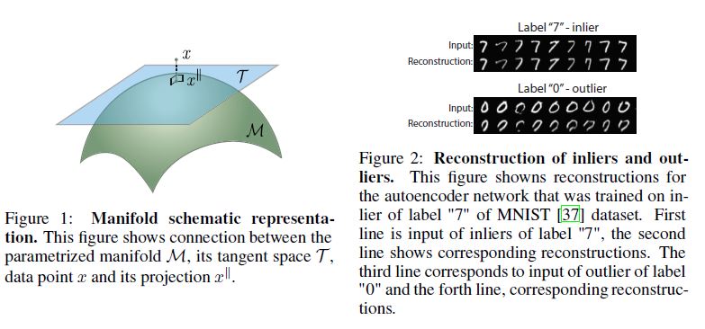
Given a new data point \(\bar{x} \in \mathbb{R^m}\), we design a novelty test to assert whether \(\bar{x}\) was sampled from model (1).
We begin by observing that \(\bar{x}\) can be non-linearly projected onto \(\bar{x}^{||} \in \mathcal{M}\) via \(\bar{x}^{||} = f(\bar{z})\), where \(\bar{z} = g(\bar{x})\).

new data point \(\bar{x} \in \mathbb{R^m}\) \(\bar{x}\)가 model (1)에서 sampled되었는지 아닌지를 주장하는 novelty test를 설계 manifold \(\mathcal{M}\)에 속하는 \(\bar{x}^{||}\)로 non-linearly projected 될 수 있는지를 관찰

Assuming \(f\) to be smooth enough, we perform a linearization based on its first-order Taylor expansion \[f(z) = f(\bar{z}) + J_{f}(\bar{z})(z − \bar{z}) + O(||z − \bar{z}||^2) , \qquad \qquad (2)\]

where \(J_f(\bar{z})\) is the Jacobi matrix computed at \(\bar{z}\), and \(\|·\|\) is the \(L_2\) norm.
We note that \(\mathcal{T}\) = span\((J_f (\bar{z}))\) represents the tangent space of \(f\) at \(\bar{x}^{||}\) that is spanned by the \(n\) independent column vectors of \(J_f(\bar{z})\), see Figure 1.
Also, we have \(\mathcal{T}\) = span(\(U^{||}\)), where \(J_f(\bar{z}) = U^{||}SV^⊤\) is the singular value decomposition (SVD) of the Jacobi matrix.
The matrix \(U^{||}\) has rank \(n\), and if we define \(U^{⊥}\) such that \(U = [U^{||}U^{⊥}]\) is a unitary matrix, we can represent the data point \(\bar{x}\) with respect to the local coordinates that define the tangent space \(\mathcal{T}\) , and its orthogonal complement \(\mathcal{T}^⊥\).

This is done by computing \[\bar{w}=U^T \bar{x} = \begin{bmatrix} U^{||^⊥}\bar{x} \\ U^{⊥^⊤}\bar{x} \end{bmatrix} = \begin{bmatrix} \bar{w}^{||} \\ \bar{w}^⊥ \end{bmatrix} \qquad \qquad \qquad (3)\]

where the rotated coordinates \(\bar{w}\) are decomposed into \(\bar{w}^{\|}\), which are parallel to \(\mathcal{T}\) , and \(\bar{w}^⊥\) which are orthogonal to \(\mathcal{T}\) .

We now indicate with \(p_X(x)\) the probability density function describing the random variable \(X\), from which training data points have been drawn.
Also, \(p_W(w)\) is the probability density function of the random variable \(W\) representing \(X\) after the change of coordinates.
The two distributions are identical.
However, we make the assumption that the coordinates \(W^{||}\), which are parallel to \(T\), and the coordinates \(W^⊥\), which are orthogonal to \(\mathcal{T}\) , are statistically independent.
This means that the following holds \[p_X(x) = p_W(w) = p_W(w^{||},w^⊥) = p_W^{||} (w^{||})p_W^⊥(w^⊥) . \qquad \qquad (4)\]

This is motivated by the fact that in (1) the noise \(ξ\) is assumed to predominantly deviate the point \(x\) away from the manifold \(\mathcal{M}\) in a direction orthogonal to \(\mathcal{T}\).
This means that \(W^⊥\) is primarely responsible for the noise effects, and since noise and drawing from the manifold are statistically independent, so are \(W^{||}\) and \(W^⊥\).

From (4), given a new data point \(\bar{x}\), we propose to perform novelty detection by executing the following test

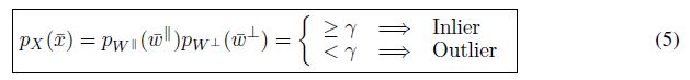
where \(\gamma\) is a suitable threshold.

3.1 Computing the distribution of data samples

The novelty detector (5) requires the computation of \(p_{W^{||}} (w^{||})\) and \(p_{W^⊥}(w^⊥)\).
Given a test data point \(\bar{x} \in \mathbb{R^m}\) its non-linear projection onto \(\mathcal{M}\) is \(\bar{x}^{||} = f(g(\bar{x}))\).
Therefore, \(\bar{w}^{||}\) can be written as \(\bar{w}^{||} = U^{||^⊤}\bar{x} = U^{||^{⊤}}(\bar{x} − \bar{x}^{||}) + U^{||^⊤} \bar{x}^{||} = U^{||^⊤}\bar{x}^{||}\), where we have made the approximation that \(U^{||^⊤}(\bar{x} − \bar{x}^{||}) ≈ 0\).
Since \(\bar{x}^{||} \in \mathcal{M}\), then in its neighborhood it can be parameterized as in (2), which means that \(w^{||}(z) = U^{||^⊤} f(\bar{z})+SV^⊤(z − \bar{z})+O(||z − \bar{z}||^2)\).
Therefore, if \(Z\) represents the random variable from which samples are drawn from the parameterized manifold, and \(p_Z(z)\) is its probability density function, then it follows that \[p_{W^{||}} (w^{||}) = |det^{S−1}| p_Z(z) , \qquad \qquad (6)\]

since \(V\) is a unitary matrix. We note that \(p_Z(z)\) is a quantity that is independent from the linearization (2), and therefore it can be learned offline, as explained in Section 5.

In order to compute \(p_{W^⊥}(w^⊥)\), we approximate it with its average over the hypersphere \(\mathcal{S}^{m−n−1}\) of radius \(\|w^{⊥}\|\), giving rise to \[p_{W^⊥}(w^⊥) ≈ \frac{\Gamma(\frac{m-n}{2})}{2\pi^{\frac{m-n}{2}}\|w^⊥\|^{m-n}}p_{\|W^⊥\|} (\|w^⊥\|), \qquad \qquad (7)\]

,where \(\Gamma(·)\) represents the gamma function.
This is motivated by the fact that noise of a given intensity will be equally present in every direction.
Moreover, its computation depends on \(p_{||W^⊥||}(||w^⊥||)\), which is the distribution of the norms of \(w^⊥\), and which can easily be learned offline by histogramming the norms of \(\bar{w}^⊥ = U^{⊥^⊤} \bar{x}\).

4 Manifold learning with adversarial autoencoders

In this section we describe the network architecture and the training procedure for learning the mapping \(f\) that define the parameterized manifold \(\mathcal{M}\), and also the mapping \(g\).
The mappings \(g\) and \(f\) represent and are modeled by an encoder network, and a decoder network, respectively.

이 section에서는 매개 변수화된 manifold \(\mathcal{M}\)을 정의하는 mapping \(f\)를 학습하기 위한 network 아키텍처 및 training 절차와 mapping \(g\)에 대해 설명한다.
mappings \(g\) 및 \(f\)는 각각 encoder network 및 decoder network에 의해 표시되고 모델링된다.

Similarly to previous work on novelty detection [38, 39, 40, 7, 11, 13], such networks are based on autoencoders [41, 42].

The autoencoder network and training should be such that they reproduce the manifold \(\mathcal{M}\) as closely as possible.
For instance, if \(\mathcal{M}\) represents the distribution of images depicting a certain object category, we would want the estimated encoder and decoder to be able to generate images as if they were drawn from the real distribution.
Differently from previous work, we require the latent space, represented by \(z\), to be close to a known distribution, preferably a normal distribution, and we would also want each of the components of \(z\) to be maximally informative, which is why we require them to be independent random variables.
Doing so facilitates learning a distribution \(p_Z(z)\) from training data mapped onto the latent space \(\Omega\).
This means that the auto-enoder has generative properties, because by sampling from \(p_Z(z)\) we would generate data points \(x \in M\).
Note that differently from GANs [29] we also require an encoder function \(g\).

autoencoder 네트워크와 training은 manifold \(\mathcal{M}\)을 가능한 가깝게 reproduce하는 것이어야 한다.
예를 들어, \(\mathcal{M}\)가 특정 객체 범주를 묘사하는 이미지의 분포distribution을 나타낸다면, 우리는 estimated된 encoder와 decoder가 real distribution에서 끌어온 것처럼 이미지를 생성할 수 있기를 원할 것이다.
이전 연구와 달리, 우리는 \(z\)로 대표되는 latent space가 known distribution에, 가급적 normal distribution에 가까울 것을 요구하고, \(z\)의 각 구성 요소가 최대한 정보를 제공하기를 원하기 때문에, independent random variables가 될 것을 요구한다.
그렇게 하면 latent space \(\Omega\)에 매핑된 training data로부터 \(p_Z(z)\) 분포를 쉽게 학습할 수 있다.
이는 auto-enoder에 generative properties이 있음을 의미하는데, 이는 \(p_Z(z)\)에서 샘플링함으로써 우리는 데이터 포인트 \(x \in M\)를 생성할 것이기 때문이다.
GANs[29]와 달리 우리는 encoder 함수 \(g\)도 필요하다.

Variational Auto-Encoders (VAEs) [44] are known to work well in presence of continuous latent variables and they can generate data from a randomly sampled latent space.
VAEs utilize stochastic variational inference and minimize the Kullback-Leibler (KL) divergence penalty to impose a prior distribution on the latent space that encourages the encoder to learn the modes of the prior distribution.
Adversarial Autoencoders (AAEs) [14], in contrast to VAEs, use an adversarial training paradigm to match the posterior distribution of the latent space with the given distribution.
One of the advantages of AAEs over VAEs is that the adversarial training procedure encourages the encoder to match the whole distribution of the prior.

Variational Auto-Encoders (VAEs)[44]는 continuous latent variables가 있는 경우 잘 작동하는 것으로 알려져 있으며 랜덤하게 샘플링된 latent space에서 data를 생성할 수 있다.
VAE는 확률적 변동 추론을 활용하고 Kullback-Libler(KL) 발산 패널티를 최소화하여 encoder가 prior distribution의 모드를 학습하도록 유도하는 latent space에 posterior distribution를 부과한다.
Adversarial Autoencoders (AAEs)[14]는 VAE와 대조적으로 적대적 훈련 패러다임을 사용하여 latent space의 posterior distribution을 given distribution과 일치시킨다.
VAE에 비해 AAE의 장점 중 하나는 적대적 훈련 절차는 encoder가 prior의 전체 distribution과 일치하도록 장려한다는 것이다.

Unfortunately, since we are concerned with working with images, both AAEs and VAEs tend to produce examples that are often far from the real data manifold.
This is because the decoder part of the network is updated only from a reconstruction loss that is typically a pixel-wise cross-entropy between input and output image.
Such loss often causes the generated images to be blurry, which has a negative effect on the proposed approach.
Similarly to AAEs, PixelGAN autoencoders [45] introduce the adversarial component to impose a prior distribution on the latent code, but the architecture is significantly different, since it is conditioned on the latent code.

안타깝게도, 우리는 이미지 작업에 관심이 있기 때문에, AAE와 VAE 모두 종종 실제 데이터 매니폴드와 거리가 먼 examples를 생성하는 경향이 있다.
이는 network의 decoder 부분이 일반적으로 input 이미지와 output 이미지 사이의 pixel-wise cross-entropy reconstruction loss에서만 업데이트되기 때문이다.
이러한 손실은 종종 생성된 이미지를 blurry하게 만들어 제안된 approach에 부정적인 영향을 미친다.
AAE와 유사하게, PixelGAN autoencoders[45]는 latent code에 prior distribution를 부과하기 위해 adversarial component를 도입하지만, latent code에 따라 조건화되기 때문에 아키텍처는 크게 다르다.

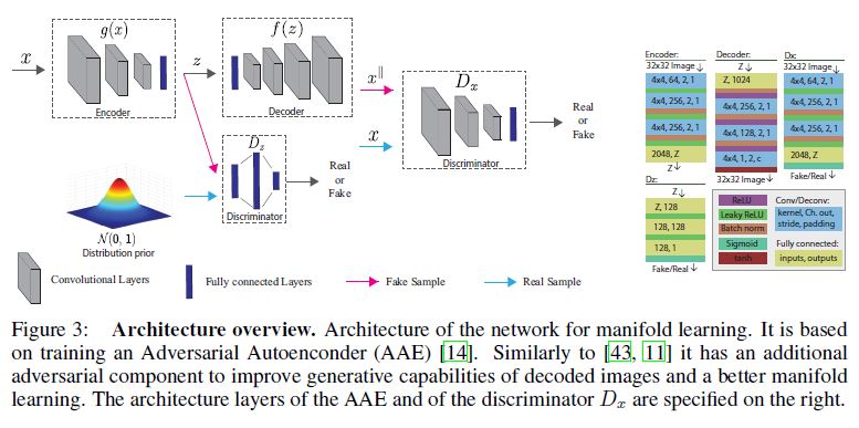
Similarly to [43, 11] we add an adversarial training criterion to match the output of the decoder with the distribution of real data.
This allows to reduce blurriness and add more local details to the generated images.
Moreover, we also combine the adversarial training criterion with AAEs, which results in having two adversarial losses: one to impose a prior on the latent space distribution, and the second one to impose a prior on the output distribution.

[43, 11]과 유사하게, 우리는 decoder의 output과 real data의 distribution을 match하기 위해 적대적 훈련 기준을 추가한다.
이렇게 하면 blurriness를 줄이고 생성된 이미지에 더 많은 local details를 추가할 수 있다.
또한 적대적 훈련 기준을 두가지 adversarial losses를 가지는 AAE와 결합한다: 하나는 latent space distribution에 prior를 부과하는 것, 둘은 output distribution에 prior를 부과하는 것.

Our full objective consists of three terms.
First, we use an adversarial loss for matching the distribution of the latent space with the prior distribution, which is a normal with 0 mean, and standard deviation 1, \(\mathcal{N}(0, 1)\).
Second, we use an adversarial loss for matching the distribution of the decoded images from \(z\) and the known, training data distribution.
Third, we use an autoencoder loss between the decoded images and the encoded input image.
Figure 3 shows the architecture configuration.

우리의 전체 목표는 세 가지 terms으로 구성되어 있다.
첫째, 우리는 평균이 0이고 표준 편차 1인 정규 분포 \(\mathcal{N}(0, 1)\)인, prior distribution를 가지는 latent space의 distribution을 일치시키기 위해 adversarial loss를 사용한다.
둘째, 우리는 \(z\)에서 디코딩된 이미지의 분포와 알려진 훈련 데이터 분포를 일치시키기 위해 adversarial loss를 사용한다.
셋째, 디코딩된 이미지와 인코딩된 입력 이미지 간에 autoencoder loss를 사용한다.
Figure 3은 아키텍처 구성을 보여줍니다.

4.1 Adversarial losses

For the discriminator \(D_z\), we use the following adversarial loss: \(\mathcal{L}_{adv−d_z} (x, g,D_z) = E[\log(D_z(\mathcal{N}(0, 1)))] + E[\log(1 − D_z(g(x)))], \qquad (8)\)

where the encoder \(g\) tries to encode \(x\) to a \(z\) with distribution close to \(\mathcal{N}(0, 1)\).
\(D_z\) aims to distinguish between the encoding produced by \(g\) and the prior normal distribution.
Hence, \(g\) tries to minimize this objective against an adversary Dz that tries to maximize it.

Similarly, we add the adversarial loss for the discriminator \(D_x\): \(\mathcal{L}_{adv−d_x}(x,D_x, f) = E[\log(D_x(x))] + E[log(1 − D_x(f(\mathcal{N}(0, 1))))] , \qquad (9)\)

where the decoder \(f\) tries to generate \(x\) from a normal distribution \(\mathcal{N}(0, 1)\), in a way that \(x\) is as if it was sampled from the real distribution.
\(D_x\) aims to distinguish between the decoding generated by \(f\) and the real data points \(x\).
Hence, \(f\) tries to minimize this objective against an adversary \(D_x\) that tries to maximize it.

4.2 Autoencoder loss

We also optimize jointly the encoder \(g\) and the decoder \(f\) so that we minimize the reconstruction error for the input \(x\) that belongs to the known data distribution. \[\mathcal{L}_{error}(x, g, f) = −E_z[\log(p(f(g(x))|x))], \qquad \qquad (10)\]

where \(\mathcal{L}_{error}\) is minus the expected log-likelihood, i.e., the reconstruction error.
This loss does not have an adversarial component but it is essential to train an autoencoder.
By minimizing this loss we encourage \(g\) and \(f\) to better approximate the real manifold.

4.3 Full objective

The combination of all the previous losses gives \[\mathcal{L}(x, g, D_z, D_x, f) = \mathcal{L}_{adv−d_z} (x, g, D_z) + \mathcal{L}_{adv−d^x}(x, D_x, f) + λ\mathcal{L}_{error}(x, g, f), \qquad \qquad (11)\]

Where \(λ\) is a parameter that strikes a balance between the reconstruction and the other losses.
The autoencoder network is obtained by minimizing (11), giving: \[\hat{g}, \hat{f} = \arg \min_{g,f} \max_{D_x,D_z} \mathcal{L}(x, g, D_z, D_x, f). \qquad \qquad (12)\]

The model is trained using stochastic gradient descent by doing alternative updates of each component as follows

• Maximize \(\mathcal{L}_{adv−d_x}\) by updating weights of \(D_x\);
• Minimize \(\mathcal{L}_{adv−d_x}\) by updating weights of \(f\);
• Maximize \(\mathcal{L}_{adv−d_z}\) by updating weights of \(D_z\);
• Minimize \(\mathcal{L}_{error}\) and \(\mathcal{L}_{adv−d_z}\) by updating weights of \(g\) and \(f\).

5 Implementation Details and Complexity

After learning the encoder and decoder networks, by mapping the training set onto the latent space through \(g\), we fit to the data a generalized Gaussian distribution and estimate \(p_Z(z)\). In addition, by histogramming the quantities \(||U^{⊥^⊤} (x − x^{||})||\) we estimate \(p_{||W^⊥||}(||w^⊥||)\). The entire training procedure takes about one hour with a high-end PC with one NVIDIA TITAN X.

When a sample is tested, the procedure entails mainly computing a derivative, i.e. the Jacoby matrix \(J_f\) , with a subsequent SVD.
\(J_f\) is computed numerically, around the test sample representation \hat{z} and takes approximately 20.4ms for an individual sample and 0.55ms if computed as part of a batch of size 512, while the SVD takes approximately 4.0ms.

6 Experiments

We evaluate our novelty detection approach, which we call Generative Probabilistic Novelty Detection (GPND), against several state-of-the-art approaches and with several performance measures.
We use the \(F_1\) measure, the area under the ROC curve (AUROC), the FPR at 95% TPR (i.e., the probability of an outlier to be misclassified as inlier), the Detection Error (i.e., the misclassification probability when TPR is 95%), and the area under the precision-recall curve (AUPR) when inliers (AUPR-In) or outliers (AUPR-Out) are specified as positives.
All reported results are from our publicly available implementation, based on the deep machine learning framework PyTorch [46].
An overview of the architecture is provided in Figure 3.

우리는 GPND(Generative Probabilitical Newnasty Detection)라고 하는 우리의 novelty detection approach을 몇 가지 최첨단 접근 방식과 몇 가지 성능 측정으로 평가한다.
우리는 \(F_1\) 측정, AUROC, the FPR at 95% TPR(즉, inlier에서 misclassified된 outlier의 probability),the Detection Error (i.e., the misclassification probability when TPR is 95%), inliers (AUPR-In) or outliers (AUPR-Out)가 positives로 구분될때 AUPR을 사용한다. 보고된 모든 결과는 deep machine learning framework PyTorch [46]를 기반으로 공개적으로 사용 가능한 구현에서 나온 것이다.
아키텍처 개요는 Figure 3에 나와 있다.

6.1 Datasets

We evaluate GPND on the following datasets.
MNIST [37] contains 70, 000 handwritten digits from 0 to 9. Each of ten categories is used as inlier class and the rest of the categories are used as outliers.

The Coil-100 dataset [47] contains 7, 200 images of 100 different objects. Each object has 72 images taken at pose intervals of 5 degrees. We downscale the images to size 32× 32. We take randomly n categories, where n ∈ 1, 4, 7 and randomly sample the rest of the categories for outliers. We repeat this procedure 30 times.

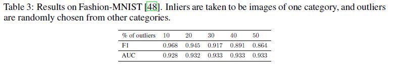
Fashion-MNIST [48] is a new dataset comprising of 28 × 28 grayscale images of 70, 000 fashion products from 10 categories, with 7, 000 images per category.
The training set has 60, 000 images and the test set has 10, 000 images. Fashion-MNIST shares the same image size, data format and the structure of training and testing splits with the original MNIST.

Others. We compare GPND with ODIN [36] using their protocol.
For inliers are used samples from CIFAR-10(CIFAR-100) [49], which is a publicly available dataset of small images of size 32×32, which have each been labeled to one of 10 (100) classes.
Each class is represented by 6, 000 (600) images for a total of 60, 000 samples.
For outliers are used samples from TinyImageNet [50], LSUN [51], and iSUN [52].
For more details please refer to [36]. We reuse the prepared datasets of outliers provided by the ODIN GitHub project page.

6.2 Results

MNIST dataset.
We follow the protocol described in [11, 7] with some differences discussed below.
Results are averages from a 5-fold cross-validation.
Each fold takes 20% of each class.
60% of each class is used for training, 20% for validation, and 20% for testing.
Once \(p_X(\hat{x})\) is computed for each validation sample, we search for the \(γ\) that gives the highest \(F_1\) measure.
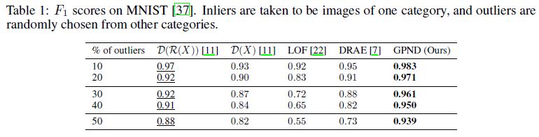
For each class of digit, we train the proposed model and simulate outliers as randomly sampled images from other categories with proportion from 10% to 50%.

MNIST dataset.
우리는 [11, 7]에 설명된 프로토콜을 따르고 아래에서 몇 가지 차이점에 대해 논의한다.
결과는 5배 교차 검증의 평균입니다.
각 접은 반의 20%를 차지합니다.
각 클래스의 60%, 검증의 20%, 테스트의 20%가 사용됩니다.
각 유효성 검사 샘플에 대해 \(p_X(\hat{x})\)가 계산되면 가장 높은 \(F_1\) 측정값을 제공하는 \(γ\)를 검색한다.
각 자릿수 클래스에 대해 제안된 모델을 교육하고 10%에서 50% 사이의 비율로 다른 범주에서 랜덤하게 샘플링된 이미지로 특이치를 시뮬레이션한다.

Results for \(\mathcal{D}(\mathcal{R}(X))\) and \(\mathcal{D}(X)\) reported in [11] correspond to the protocol for which data is not split into separate training, validation and testing sets, meaning that the same inliers used for training were also used for testing.
We diverge from this protocol and do not reuse the same inliers for training and testing.
We follow the 60%/20%/20% splits for training, validation and testing.
This makes our testing harder, but more realistic, while we still compare our numbers against those obtained by others with easier settings.
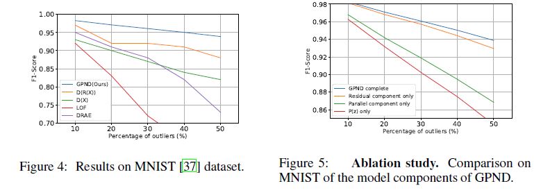
Results on the MNIST dataset are shown in Table 1 and Figure 4, where we compare with [11, 22, 7].

[11]에 보고된 \(\mathcal{D}(\mathcal{R)(X)\) 및 \(\mathcal{D}(X)\)에 대한 결과는 데이터가 별도의 훈련, 유효성 검사 및 테스트 세트로 분할되지 않는 프로토콜에 해당하며, 이는 훈련에 사용된 것과 동일한 한정자가 테스트에도 사용되었음을 의미한다.
우리는 이 프로토콜에서 벗어나 훈련과 테스트를 위해 동일한 이니셜을 재사용하지 않는다.
우리는 훈련, 검증 및 테스트를 위해 60%/20%/20% 분할을 따른다.
이것은 우리의 시험을 더 어렵지만 더 현실적이게 만들지만, 우리는 여전히 더 쉬운 설정을 가진 다른 사람들에 의해 얻어진 숫자와 비교한다.
MNIST 데이터 세트에 대한 결과는 표 1과 그림 4에 나타나 있으며, 여기서 우리는 [11, 22, 7]과 비교한다.

Coil-100 dataset.
We follow the protocol described in [8] with some differences discussed below.
Results are averages from 5-fold cross-validation.
Each fold takes 20% of each class.
Because the count of samples per category is very small, we use 80% of each class for training, and 20% for testing.
We find the optimal threshold \(γ\) on the training set.
Results reported in [8] correspond to not splitting data into separate training, validation and testing sets, because it is not essential, since they leverage a VGG [53] network pretrained on ImageNet [54].
We diverge from that protocol and do not reuse inliers and follow 80%/20% splits for training and testing.

Coil-100 dataset.
우리는 [8]에 설명된 프로토콜을 따르고 아래에서 몇 가지 차이점에 대해 논의한다.
결과는 5배 교차 검증의 평균입니다.
각 접은 반의 20%를 차지합니다.
범주당 샘플의 수가 매우 적기 때문에, 우리는 각 클래스의 80%, 테스트에 20%를 사용합니다.
우리는 훈련 세트에서 최적의 임계값 \(γ\)를 찾는다.
[8]에 보고된 결과는 ImageNet [54]에서 사전 훈련된 VGG [53] 네트워크를 활용하기 때문에 반드시 필요한 것은 아니기 때문에 데이터를 별도의 교육, 검증 및 테스트 세트로 분할하지 않는 것과 일치한다.
우리는 그 프로토콜에서 벗어나서 특이치를 재사용하지 않으며 훈련과 테스트를 위해 80%/20% 분할을 따른다.

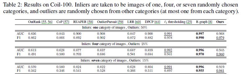
Results on Coil-100 are shown in Table 2.
We do not outperform R-graph [8], however as mentioned before, R-graph uses a pretrained VGG network, while we train an autoencoder from scratch on a very limited number of samples, which is on average only 70 per category.

코일-100에 대한 결과는 표 2에 나와 있습니다.
우리는 R-그래프[8]를 능가하지 않지만, 앞에서 언급한 바와 같이, R-그래프는 사전 훈련된 VGG 네트워크를 사용하는 반면, 우리는 범주당 평균 70개에 불과한 매우 제한된 수의 샘플에서 자동 인코더를 처음부터 훈련시킨다.

Fashion-MNIST dataset.
We repeat the same experiment with the same protocol that we have used for MNIST, but on Fashion-MNIST. Results are provided in Table 3.

Fashion-MNIST dataset. 우리는 MNIST에 사용한 것과 동일한 프로토콜로 동일한 실험을 반복하지만, 패션-MNIST에 대해서는 같은 실험을 반복한다. 결과는 표 3에 제시되어 있다.

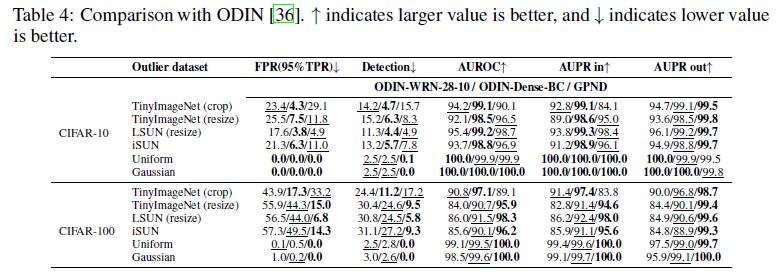
CIFAR-10 (CIFAR-100) dataset.
We follow the protocol described in [36], where for inliers and outliers are used different datasets. ODIN relies on a pretrained classifier and thus requires label information provided with the training samples, while our approach does not use label information.
The results are reported in Table 4. Despite the fact that ODIN relies upon powerful classifier networks such as Dense-BC and WRN with more than 100 layers, the much smaller network of GPND competes well with ODIN.
Note that for CIFAR-100, GPND significantly outperforms both ODIN architectures.
We think this might be due to the fact that ODIN relies on the perturbation of the network classifier output, which becomes less accurate as the number of classes grows from 10 to 100.
On the other hand, GPND does not use class label information and copes much better with the additional complexity induced by the increased number of classes.

CIFAR-10 (CIFAR-100) dataset.
우리는 [36]에 설명된 프로토콜을 따르는데, 여기서 특이치와 특이치는 서로 다른 데이터 세트를 사용한다. ODIN은 사전 훈련된 분류기에 의존하므로 훈련 샘플과 함께 제공되는 라벨 정보가 필요한 반면, 우리의 접근 방식은 라벨 정보를 사용하지 않는다.
결과는 표 4에 보고된다. ODIN이 100개 이상의 계층을 가진 Dense-BC 및 WRN과 같은 강력한 분류기 네트워크에 의존한다는 사실에도 불구하고, GPN의 훨씬 더 작은 네트워크는 ODIN과 잘 경쟁한다.
CIFAR-100의 경우 GPND가 두 ODIN 아키텍처를 크게 능가한다는 점에 유의한다.
이는 ODIN이 네트워크 분류기 출력의 섭동에 의존하기 때문일 수 있으며, 클래스 수가 10개에서 100개로 증가함에 따라 정확도가 낮아진다.
반면, GPND는 클래스 레이블 정보를 사용하지 않으며 클래스 수에 의해 유발되는 추가적인 복잡성으로 훨씬 더 잘 대처한다.

6.3 Ablation

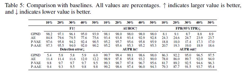
Table 5 compares GPND with some baselines to better appreciate the improvement provided by the architectural choices.
The baselines are:
i) vanilla AE with thresholding of the reconstruction error and same pipeline (AE);
ii) proposed approach where the AAE is replaced by a VAE (P-VAE);
iii) proposed approach where the AAE is without the additional adversarial component induced by the discriminator applied to the decoded image (P-AAE).

표 5는 구조 선택에 의해 제공되는 개선을 더 잘 평가하기 위해 GPND를 일부 기준선과 비교한다.
기준선은 다음과 같습니다.
i) 재구성 오류의 임계값과 동일한 파이프라인(AE)을 가진 바닐라 AE;
ii) AAE가 VAE(P-VAE)로 대체되는 경우 제안된 접근 방식
iii) AAE가 디코딩된 영상(P-AAE)에 적용된 판별기에 의해 유도된 추가 적대적 구성 요소 없이 제안된 접근법이다.

To motivate the importance of each component of \(p_X(\hat{x})\) in (5), we repeat the experiment with MNIST under the following conditions:
a) GPND Complete is the unmodified approach, where \(p_X(\hat{x})\) is computed as in (5);
b) Parallel component only drops \(p_{W^⊥}\) and assumes \(p_X(\hat{x}) = p_{W^{||}} (\hat{w}^{||}); c)\) Perpendicular component only drops \(p_{W^{||}}\) and assumes \(p_X(\hat{x}) = p_{W^⊥}(\hat{w}^⊥); d) p_Z(z)\) only drops also \(|detS^{−1}|\) and assumes \(p_X(\hat{x}) = p_Z(z)\).
dThe results are shown in Figure 5.
It can be noticed that the scaling factor \(|detS^{−1}|\) plays an essential role in the Parallel component only, and that the Parallel component only and the Perpendicular component only play an essential role in composing the GPND Complete model.

Additional implementation details include the choice of hyperparameters.
For MNIST and COIL-100 the latent space size was chosen to maximize \(F_1\) on the validation set.
It is 16, and we varied it from 16 to 64 without significant performance change.
For CIFAR-10 and CIFAR-100, the latent space size was set to 256.
The hyperparameters of all losses are one, except for \(L_{error}\) and \(L_{adv−d_z}\) when optimizing forDz, which are equal to 2.0.
For CIFAR-10 and CIFAR-100, the hyperparameter of \(L_{error}\) is 10.0.
We use the Adam optimizer with learning rate of 0.002, batch size of 128, and 80 epochs.

7 Conclusion

We introduced GPND, an approach and a network architecture for novelty detection that is based on learning mappings \(f\) and \(g\) that define the parameterized manifold \(\mathcal{M}\) which captures the underlying structure of the inlier distribution.
Unlike prior deep learning based methods, GPND detects that a given sample is an outlier by evaluating its inlier probability distribution.
We have shown how each architectural and model components are essential to the novelty detection.
In addition, with a relatively simple architecture we have shown how GPND provides state-of-the-art performance using different measures, different datasets, and different protocols, demonstrating to compare favorably also with the out-of-distribution literature.

inlier distribution의 underlying structure를 포착하는 매개 변수화된 매니폴드 \(\mathcal{M}\)를 정의하는 학습 매핑 \(f\)와 \(g\)를 기반으로 하는 novelty detection을 위한 approach 및 network 아키텍처인 GPND를 소개했다.
이전의 deep learning based method과 달리, GPND는 inlier probability distribution를 평가하여 주어진 sample이 outlier임을 감지한다.
우리는 각 아키텍처 및 모델 components가 novelty detection에 어떻게 필수적인지 보여주었다.
또한, 우리는 비교적 간단한 아키텍처를 사용하여 GPND가 다른 measures, 다른 datasets, 다른 protocols을 사용하여 어떻게 state-of-the-art performance를 제공하는지를 보여 주었으며, out-of-distribution literature과도 잘 비교되는 것을 보여주었다.

Acknowledgments

This material is based upon work supported by the National Science Foundation under Grant No. IIS-1761792.